0%

吴恩达《深度学习专项》代码实战(十):3.用 NumPy 复现参数一致的 torch.conv2d 前向传播

《深度学习专项》只介绍了卷积的stride, padding这两个参数。实际上,编程框架中常用的卷积还有其他几个参数。在这篇文章里,我会介绍如何用NumPy复现PyTorch中的二维卷积torch.conv2d的前向传播。如果大家也想多学一点的话,建议看完本文后也自己动手写一遍卷积,彻底理解卷积中常见的参数。

项目网址:https://github.com/SingleZombie/DL-Demos/tree/master/dldemos/BasicCNN

本文代码在dldemos/BasicCNN/np_conv.py这个文件里。

卷积参数介绍

torch.conv2d类似,在这份实现中,我们的卷积应该有类似如下的函数定义(张量的形状写在docstring中):

1
2
3
4
5
6
7
8
9
10
11
12
13
14
15
16
17
18
19
20
21
22
23
def conv2d(input: np.ndarray,
weight: np.ndarray,
stride: int,
padding: int,
dilation: int,
groups: int,
bias: np.ndarray = None) -> np.ndarray:
"""2D Convolution Implemented with NumPy

Args:
input (np.ndarray): The input NumPy array of shape (H, W, C).
weight (np.ndarray): The weight NumPy array of shape
(C', F, F, C / groups).
stride (int): Stride for convolution.
padding (int): The count of zeros to pad on both sides.
dilation (int): The space between kernel elements.
groups (int): Split the input to groups.
bias (np.ndarray | None): The bias NumPy array of shape (C').
Default: None.

Outputs:
np.ndarray: The output NumPy array of shape (H', W', C')
"""

我们知道,对于不加任何参数的卷积,其计算方式如下:

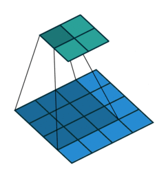
此图中,下面蓝色的区域是一张$4 \times 4$的输入图片,输入图片上深蓝色的区域是一个$3 \times 3$的卷积核。这样,会生成上面那个$2 \times 2$的绿色的输出图片。每轮计算输出图片上一个深绿色的元素时,卷积核所在位置会标出来。

接下来,使用类似图例,我们来看看卷积各参数的详细解释。

stride(步幅)

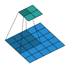
每轮计算后,卷积核向右或向下移动多格,而不仅仅是1格。每轮移动的格子数用stride表示。上图是stride=2的情况。

padding(填充数)

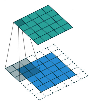
卷积开始前,向输入图片四周填充数字(最常见的情况是填充0),填充的数字个数用padding表示。这样,输出图片的边长会更大一些。一般我们会为了让输出图片和输入图片一样大而调整padding,比如上图那种padding=1的情况。

dilation(扩充数)

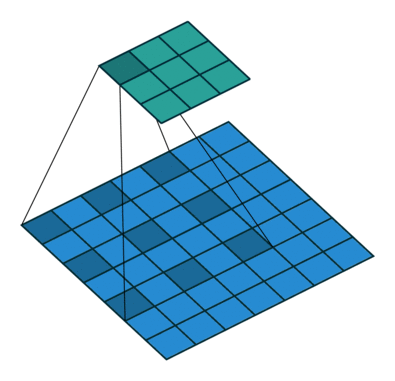
被卷积的相邻像素之间有间隔,这个间隔等于dilation。等价于在卷积核相邻位置之间填0,再做普通的卷积。上图是dilation=2的情况。

dliated convolution 被翻译成空洞卷积。

groups(分组数)

下图展示了输入通道数12,输出通道数6的卷积在两种不同groups下的情况。左边是group=1的普通卷积,右边是groups=3的分组卷积。在具体看分组卷积的介绍前,大家可以先仔细观察这张图,看看能不能猜出分组卷积是怎么运算的。

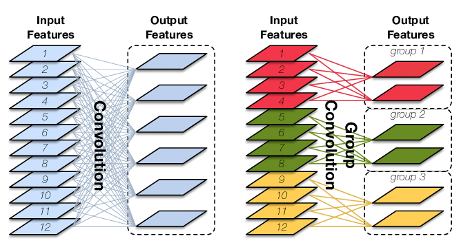
当输入图片有多个通道时,卷积核也应该有相同数量的通道。输入图片的形状是(H, W, C)的话,卷积核的形状就应该是(f, f, C)。

但是,这样一轮运算只能算出一张单通道的图片。为了算多通道的图片,应该使用多个卷积核。因此,如果输入图片的形状是(H, W, C),想要生成(H, W, C’)的输出图片,则应该有C’个形状为(f, f, C)的卷积核,或者说卷积核组的形状是(C’, f, f, C)。

如分组卷积示意图的左图所示,对于普通卷积,每一个输出通道都需要用到所有输入通道的数据。为了减少计算量,我们可以把输入通道和输出通道分组。每组的输出通道仅由该组的输入通道决定。如示意图的右图所示,我们令分组数groups=3,这样,一共有6个卷积核,每组的输入通道有4个,输出通道有2个(即使用2个卷积核)。这时候,卷积核组的形状应该是(C’=6, f, f, C=4)。

groups最常见的应用是令groups=C,即depth-wise convolution。《深度学习专项》第四门课第二周会介绍有关的知识。

代码实现

理解了所有参数,下面让我们来用NumPy实现这样一个卷积。

完整的代码是:

1
2
3
4
5
6
7
8
9
10
11
12
13
14
15
16
17
18
19
20
21
22
23
24
25
26
27
28
29
30
31
32
33
34
35
36
37
38
39
40
41
42
43
44
45
46
47
48
49
50
51
52
53
54
55
56
57
58
59
60
61
62
63
64
65
66
67
68
69
70
71
72
73
def conv2d(input: np.ndarray,
weight: np.ndarray,
stride: int,
padding: int,
dilation: int,
groups: int,
bias: np.ndarray = None) -> np.ndarray:
"""2D Convolution Implemented with NumPy

Args:
input (np.ndarray): The input NumPy array of shape (H, W, C).
weight (np.ndarray): The weight NumPy array of shape
(C', F, F, C / groups).
stride (int): Stride for convolution.
padding (int): The count of zeros to pad on both sides.
dilation (int): The space between kernel elements.
groups (int): Split the input to groups.
bias (np.ndarray | None): The bias NumPy array of shape (C').
Default: None.

Outputs:
np.ndarray: The output NumPy array of shape (H', W', C')
"""
h_i, w_i, c_i = input.shape
c_o, f, f_2, c_k = weight.shape

assert (f == f_2)
assert (c_i % groups == 0)
assert (c_o % groups == 0)
assert (c_i // groups == c_k)
if bias is not None:
assert (bias.shape[0] == c_o)

f_new = f + (f - 1) * (dilation - 1)
weight_new = np.zeros((c_o, f_new, f_new, c_k), dtype=weight.dtype)
for i_c_o in range(c_o):
for i_c_k in range(c_k):
for i_f in range(f):
for j_f in range(f):
i_f_new = i_f * dilation
j_f_new = j_f * dilation
weight_new[i_c_o, i_f_new, j_f_new, i_c_k] = \
weight[i_c_o, i_f, j_f, i_c_k]

input_pad = np.pad(input, [(padding, padding), (padding, padding), (0, 0)])

def cal_new_sidelngth(sl, s, f, p):
return (sl + 2 * p - f) // s + 1

h_o = cal_new_sidelngth(h_i, stride, f_new, padding)
w_o = cal_new_sidelngth(w_i, stride, f_new, padding)

output = np.empty((h_o, w_o, c_o), dtype=input.dtype)

c_o_per_group = c_o // groups

for i_h in range(h_o):
for i_w in range(w_o):
for i_c in range(c_o):
i_g = i_c // c_o_per_group
h_lower = i_h * stride
h_upper = i_h * stride + f_new
w_lower = i_w * stride
w_upper = i_w * stride + f_new
c_lower = i_g * c_k
c_upper = (i_g + 1) * c_k
input_slice = input_pad[h_lower:h_upper, w_lower:w_upper,
c_lower:c_upper]
kernel_slice = weight_new[i_c]
output[i_h, i_w, i_c] = np.sum(input_slice * kernel_slice)
if bias:
output[i_h, i_w, i_c] += bias[i_c]
return output

先回顾一下我们要用到的参数。

1
2
3
4
5
6
7
def conv2d(input: np.ndarray,
weight: np.ndarray,
stride: int,
padding: int,
dilation: int,
groups: int,
bias: np.ndarray = None) -> np.ndarray:

再次提醒,input的形状是(H, W, C),卷积核组weight的形状是(C', H, W, C_k)。其中C_k = C / groups。同时C'也必须能够被groups整除。bias的形状是(C')

一开始,把要用到的形状从shape里取出来,并检查一下形状是否满足要求。

1
2
3
4
5
6
7
8
9
h_i, w_i, c_i = input.shape
c_o, f, f_2, c_k = weight.shape

assert (f == f_2)
assert (c_i % groups == 0)
assert (c_o % groups == 0)
assert (c_i // groups == c_k)
if bias is not None:
assert (bias.shape[0] == c_o)

回忆一下,空洞卷积可以用卷积核扩充实现。因此,在开始卷积前,可以先预处理好扩充后的卷积核。我们先算好扩充后卷积核的形状,并创建好新的卷积核,最后用多重循环给新卷积核赋值。

1
2
3
4
5
6
7
8
9
10
f_new = f + (f - 1) * (dilation - 1)
weight_new = np.zeros((c_o, f_new, f_new, c_k), dtype=weight.dtype)
for i_c_o in range(c_o):
for i_c_k in range(c_k):
for i_f in range(f):
for j_f in range(f):
i_f_new = i_f * dilation
j_f_new = j_f * dilation
weight_new[i_c_o, i_f_new, j_f_new, i_c_k] = \
weight[i_c_o, i_f, j_f, i_c_k]

接下来,我们要考虑padding。np.pad就是填充操作使用的函数。该函数第一个参数是输入,第二个参数是填充数量,要分别写出每个维度上左上和右下的填充数量。我们只填充图片的前两维,并且左上和右下填的数量一样多。因此,填充的写法如下:

1
input_pad = np.pad(input, [(padding, padding), (padding, padding), (0, 0)])

预处理都做好了,马上要开始卷积计算了。在计算开始前,我们还要把算出输出张量的形状并将其初始化。

1
2
3
4
5
6
7
def cal_new_sidelngth(sl, s, f, p):
return (sl + 2 * p - f) // s + 1

h_o = cal_new_sidelngth(h_i, stride, f_new, padding)
w_o = cal_new_sidelngth(w_i, stride, f_new, padding)

output = np.empty((h_o, w_o, c_o), dtype=input.dtype)

为严谨起见,我这里用统一的函数计算了卷积后的宽高。不考虑dilation的边长公式由cal_new_sidelngth表示。如果对这个公式不理解,可以自己推一推。而考虑dilation时,只需要把原来的卷积核长度f换成新卷积核长度f_new即可。

初始化output时,我没有像前面初始化weight_new一样使用np.zeros,而是用了np.empty。这是因为weight_new会有一些地方不被访问到,这些地方都应该填0。而output每一个元素都会被访问到并赋值,可以不用令它们初值为0。理论上,np.empty这种不限制初值的初始化方式是最快的,只是使用时一定别忘了要先给每个元素赋值。这种严谨的算法实现思维还是挺重要的,尤其是在用C++实现高性能的底层算法时。

终于,可以进行卷积计算了。这部分的代码如下:

1
2
3
4
5
6
7
8
9
10
11
12
13
14
15
16
17
18
c_o_per_group = c_o // groups

for i_h in range(h_o):
for i_w in range(w_o):
for i_c in range(c_o):
i_g = i_c // c_o_per_group
h_lower = i_h * stride
h_upper = i_h * stride + f_new
w_lower = i_w * stride
w_upper = i_w * stride + f_new
c_lower = i_g * c_k
c_upper = (i_g + 1) * c_k
input_slice = input_pad[h_lower:h_upper, w_lower:w_upper,
c_lower:c_upper]
kernel_slice = weight_new[i_c]
output[i_h, i_w, i_c] = np.sum(input_slice * kernel_slice)
if bias:
output[i_h, i_w, i_c] += bias[i_c]

来一点一点看这段代码。

c_o_per_group = c_o // groups预处理了每组的输出通道数,后面会用到这个数。

为了填入输出张量每一处的值,我们应该遍历输出张量的每一个元素的下标:

1
2
3
for i_h in range(h_o):
for i_w in range(w_o):
for i_c in range(c_o):

做卷积时,我们要获取两个东西:被卷积的原图像上的数据、卷积用的卷积核。所以,下一步应该去获取原图像上的数据切片。这个切片可以这样表示

1
2
input_slice = input_pad[h_lower:h_upper, w_lower:w_upper,
c_lower:c_upper]

宽和高上的截取范围很好计算。只要根据stride确认截取起点,再加上f_new就得到了截取终点。

1
2
3
4
h_lower = i_h * stride
h_upper = i_h * stride + f_new
w_lower = i_w * stride
w_upper = i_w * stride + f_new

比较难想的是考虑groups后,通道上的截取范围该怎么获得。这里,不妨再看一次分组卷积的示意图:

获取通道上的截取范围,就是获取右边那幅图中的输入通道组。究竟是红色的1-4,还是绿色的5-8,还是黄色的9-12。为了知道是哪一个范围,我们要算出当前输出通道对应的组号(颜色),这个组号由下面的算式获得:

1
i_g = i_c // c_o_per_group

有了组号,就可以方便地计算通道上的截取范围了。

1
2
c_lower = i_g * c_k
c_upper = (i_g + 1) * c_k

整个获取输入切片的代码如下:

1
2
3
4
5
6
7
8
9
i_g = i_c // c_o_per_group
h_lower = i_h * stride
h_upper = i_h * stride + f_new
w_lower = i_w * stride
w_upper = i_w * stride + f_new
c_lower = i_g * c_k
c_upper = (i_g + 1) * c_k
input_slice = input_pad[h_lower:h_upper, w_lower:w_upper,
c_lower:c_upper]

而卷积核就很容易获取了,直接选中第i_c个卷积核即可:

1
kernel_slice = weight_new[i_c]

最后是卷积运算,别忘了加上bias。

1
2
3
output[i_h, i_w, i_c] = np.sum(input_slice * kernel_slice)
if bias:
output[i_h, i_w, i_c] += bias[i_c]

写完了所有东西,返回输出结果。

1
return output

单元测试

为了方便地进行单元测试,我使用了pytest这个单元测试库。可以直接pip一键安装:

1
pip install pytest

之后就可以用pytest执行我的这份代码,代码里所有以test_开头的函数会被认为是单元测试的主函数。

1
pytest dldemos/BasicCNN/np_conv.py

完整代码如下:

1
2
3
4
5
6
7
8
9
10
11
12
13
14
15
16
17
18
19
20
21
22
23
24
25
26
27
28
29
30
31
32
33
34
@pytest.mark.parametrize('c_i, c_o', [(3, 6), (2, 2)])
@pytest.mark.parametrize('kernel_size', [3, 5])
@pytest.mark.parametrize('stride', [1, 2])
@pytest.mark.parametrize('padding', [0, 1])
@pytest.mark.parametrize('dilation', [1, 2])
@pytest.mark.parametrize('groups', ['1', 'all'])
@pytest.mark.parametrize('bias', [False])
def test_conv(c_i: int, c_o: int, kernel_size: int, stride: int, padding: str,
dilation: int, groups: str, bias: bool):
if groups == '1':
groups = 1
elif groups == 'all':
groups = c_i

if bias:
bias = np.random.randn(c_o)
torch_bias = torch.from_numpy(bias)
else:
bias = None
torch_bias = None

input = np.random.randn(20, 20, c_i)
weight = np.random.randn(c_o, kernel_size, kernel_size, c_i // groups)

torch_input = torch.from_numpy(np.transpose(input, (2, 0, 1))).unsqueeze(0)
torch_weight = torch.from_numpy(np.transpose(weight, (0, 3, 1, 2)))
torch_output = torch.conv2d(torch_input, torch_weight, torch_bias, stride,
padding, dilation, groups).numpy()
torch_output = np.transpose(torch_output.squeeze(0), (1, 2, 0))

numpy_output = conv2d(input, weight, stride, padding, dilation, groups,
bias)

assert np.allclose(torch_output, numpy_output)

其中,单元测试函数的定义如下:

1
2
3
4
5
6
7
8
9
@pytest.mark.parametrize('c_i, c_o', [(3, 6), (2, 2)])
@pytest.mark.parametrize('kernel_size', [3, 5])
@pytest.mark.parametrize('stride', [1, 2])
@pytest.mark.parametrize('padding', [0, 1])
@pytest.mark.parametrize('dilation', [1, 2])
@pytest.mark.parametrize('groups', ['1', 'all'])
@pytest.mark.parametrize('bias', [False])
def test_conv(c_i: int, c_o: int, kernel_size: int, stride: int, padding: str,
dilation: int, groups: str, bias: bool):

先别管上面那一堆装饰器,先看一下单元测试中的输入参数。在对某个函数进行单元测试时,要测试该函数的参数在不同取值下的表现。我打算测试我们的conv2d在各种输入通道数、输出通道数、卷积核大小、步幅、填充数、扩充数、分组数、是否加入bias的情况。

@pytest.mark.parametrize用于设置单元测试参数的可选值。我设置了6组参数,每组参数有2个可选值,经过排列组合后可以生成2^6=64个单元测试,pytest会自动帮我们执行不同的测试。

在测试函数内,我先预处理了一下输入的参数,并生成了随机的输入张量,使这些参数和conv2d的参数一致。

1
2
3
4
5
6
7
8
9
10
11
12
13
14
15
16
def test_conv(c_i: int, c_o: int, kernel_size: int, stride: int, padding: str,
dilation: int, groups: str, bias: bool):
if groups == '1':
groups = 1
elif groups == 'all':
groups = c_i

if bias:
bias = np.random.randn(c_o)
torch_bias = torch.from_numpy(bias)
else:
bias = None
torch_bias = None

input = np.random.randn(20, 20, c_i)
weight = np.random.randn(c_o, kernel_size, kernel_size, c_i // groups)

为了确保我们实现的卷积和torch.conv2d是对齐的,我们要用torch.conv2d算一个结果,作为正确的参考值。

1
2
3
4
5
torch_input = torch.from_numpy(np.transpose(input, (2, 0, 1))).unsqueeze(0)
torch_weight = torch.from_numpy(np.transpose(weight, (0, 3, 1, 2)))
torch_output = torch.conv2d(torch_input, torch_weight, torch_bias, stride,
padding, dilation, groups).numpy()
torch_output = np.transpose(torch_output.squeeze(0), (1, 2, 0))

由于torch里张量的形状格式是NCHW,weight的形状是C’Cff,我这里做了一些形状上的转换。

之后,调用我们自己的卷积函数:

1
2
numpy_output = conv2d(input, weight, stride, padding, dilation, groups,
bias)

最后,验证一下两个结果是否对齐:

1
assert np.allclose(torch_output, numpy_output)

运行前面提到的单元测试命令,pytest会输出很多测试的结果。

1
pytest dldemos/BasicCNN/np_conv.py

如果看到了类似的输出,就说明我们的代码是正确的。

1
========== 64 passed in 1.20s ===============

总结

在这篇文章中,我介绍了torch.conv2d的等价NumPy实现。同时,我还详细说明了卷积各参数(stride, padding, dilation, groups)的意义。通过阅读本文,相信大家能够深刻地理解一轮卷积是怎么完成的。

如果你也想把这方面的基础打牢,一定一定要自己动手从头写一份代码。在写代码,调bug的过程中,一定会有很多收获。

相比torch里的卷积,这份卷积实现还不够灵活。torch里可以自由输入卷积核的宽高、stride的宽高。而我们默认卷积核是正方形,宽度和高度上的stride是一样的。不过,要让卷积更灵活一点,只需要稍微修改一些预处理数据的代码即可,卷积的核心实现代码是不变的。

其实,在编程框架中,卷积的实现都是很高效的,不可能像我们这样先扩充卷积核,再填充输入图像。这些操作都会引入很多冗余的计算量。为了尽可能利用并行加速卷积的运算,卷积的GPU实现使用了一种叫做im2col的算法。这种算法会把每次卷积乘加用到的输入图像上的数据都放进列向量中,把卷积乘加转换成一次矩阵乘法。有兴趣的话欢迎搜索这方面的知识。

这篇文章仅介绍了卷积操作的正向传播。有了正向传播,反向传播倒没那么了难了。之后有时间的话我会再分享一篇用NumPy实现卷积反向传播的文章。

参考资料

本文中的动图来自于 https://github.com/vdumoulin/conv_arithmetic

本文中分组卷积的图来自于论文 https://www.researchgate.net/publication/321325862_CondenseNet_An_Efficient_DenseNet_using_Learned_Group_Convolutions