Yifan Zhou's Blog

The quadratic $O(N^2)$ complexity of self-attention has long been a major computational bottleneck in modern large models. This year, one of the most active directions for improving attention mechanisms has been sparse attention: instead of attending to all key–value (KV) tokens, each query attends only to a small subset of important tokens. Representative works in this direction include MoBA from Kimi and NSA from DeepSeek.

However, despite their sparsity, these methods do not fundamentally reduce the asymptotic complexity of attention. Their overall runtime still grows with sequence length $N$ following an $O(N^2)$ trend.

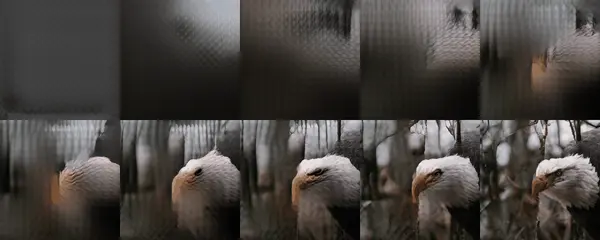
To address this limitation, our recent work, Log-linear Sparse Attention (LLSA), reduces the complexity of sparse attention to $O(N \log N)$ at the algorithmic level. In addition, we provide a highly optimized Triton implementation of LLSA tailored to modern GPU architectures, and employ efficient sparse algorithms to minimize the overhead introduced by sparsity itself. We validate the effectiveness of LLSA on pure pixel-space DiT generation tasks without VAE and without patchification. On pixel sequences as long as $512 \times 512$, LLSA achieves generation quality comparable to full attention, while significantly reducing computation time.

In this blog post, I introduce our arXiv paper Trainable Log-linear Sparse Attention for Efficient Diffusion Transformers, and conclude with my own assessment of the work and possible future directions. Our high-performance Triton implementation of LLSA has also been open-sourced. We warmly welcome fellow researchers to use our method, and to discuss or collaborate with us after reading the paper.

arXiv: https://arxiv.org/abs/2512.16615
GitHub: https://github.com/SingleZombie/LLSA

Background

First, let us clarify the scope of LLSA. As stated in the paper title, LLSA is a trainable attention mechanism. Therefore, it differs fundamentally from inference-time acceleration methods for pretrained models such as Sparse VideoGen. LLSA does not aim to approximate full attention outputs as closely as possible; instead, it only needs to enable successful training of Transformers equipped with this attention mechanism. In this sense, LLSA is more directly comparable to mechanisms such as MoBA (Mixture of Block Attention) and NSA (Native Sparse Attention), and enjoys a much larger design space.

In this section, I first provide background to clarify the problem we aim to solve, and then briefly review related prior work.

Sparsifying Attention

The attention operation can be written as

Here, $\mathbf{Q}, \mathbf{K}, \mathbf{V} \in \mathbb{R}^{N \times d}$, where $N$ is the sequence length and $d$ is the feature dimension. We refer to these as queries, keys, and values.

This formulation aggregates $N$ queries into matrix form. If we consider a single query $q \in \mathbb{R}^{1 \times d}$, the operation is easier to interpret: we compute normalized similarities $p = \text{softmax}(q\mathbf{K}^{\intercal})$, then obtain the attention output $o = p\mathbf{V}$. Concatenating all $o$ yields the final output $\mathbf{O}$.

From a complexity perspective, standard full attention is slow because each of the $N$ queries attends to all $N$ keys and values, resulting in $O(N^2)$ complexity. Equivalently, the matrix multiplication $\mathbf{Q}\mathbf{K}^{\intercal}$ has complexity $O(N^2 d)$, which reduces to $O(N^2)$ when $d$ is treated as a constant. As sequence length increases, attention quickly dominates runtime compared to linear-time components such as MLPs or normalization layers.

Many studies have observed that attention matrices $\mathbf{P}$ in pretrained models are sparse: for each query, most key similarities are close to zero and can be ignored. This naturally leads to the idea of Top-$K$ attention—selecting only the $K$ most important keys and values per query.

While this idea is correct in principle, it does not automatically lead to acceleration. To find the Top-$K$, one must first compute all $O(N^2)$ query–key similarities. If those similarities are already computed, applying sparsity afterward provides little benefit. Thus, Top-$K$ sparse attention can only be efficient if query–key similarities can themselves be computed efficiently.

Modern Top-$K$ sparse attention methods therefore rely on approximate similarity estimation. To understand them, we first review Block Sparse FlashAttention.

Block Sparse FlashAttention

Modern GPU programming is fundamentally based on parallelism: a GPU can process $B$ identical operations simultaneously. For example, when summing two vectors of length $N$, we do not write a loop of length $N$ that processes one element at a time; instead, we process $B$ elements per iteration using a loop of length $N/B$.

FlashAttention adopts this principle by performing attention computation in blocks. Suppose $\mathbf{Q}, \mathbf{K}, \mathbf{V}$ are partitioned into $N/B$ blocks, where block $i$ contains $\mathbf{Q}_i, \mathbf{K}_i, \mathbf{V}_i \in \mathbb{R}^{B \times d}$. We can then launch $N/B$ programs, each computing outputs $\mathbf{O}_i$ for one query block. Inside each program, a loop of length $N/B$ iterates over key–value blocks.

This structure naturally supports block sparsity. If a sparse algorithm determines that $\mathbf{Q}_i$ does not need to attend to $\mathbf{K}_j$, the $j$-th iteration of the $i$-th program can be skipped. The choice of sparsity pattern is unrestricted—for example, sliding-window attention.

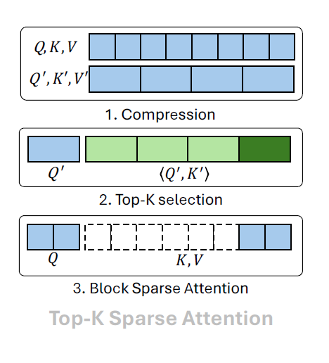
Top-$K$ Block Sparse Attention

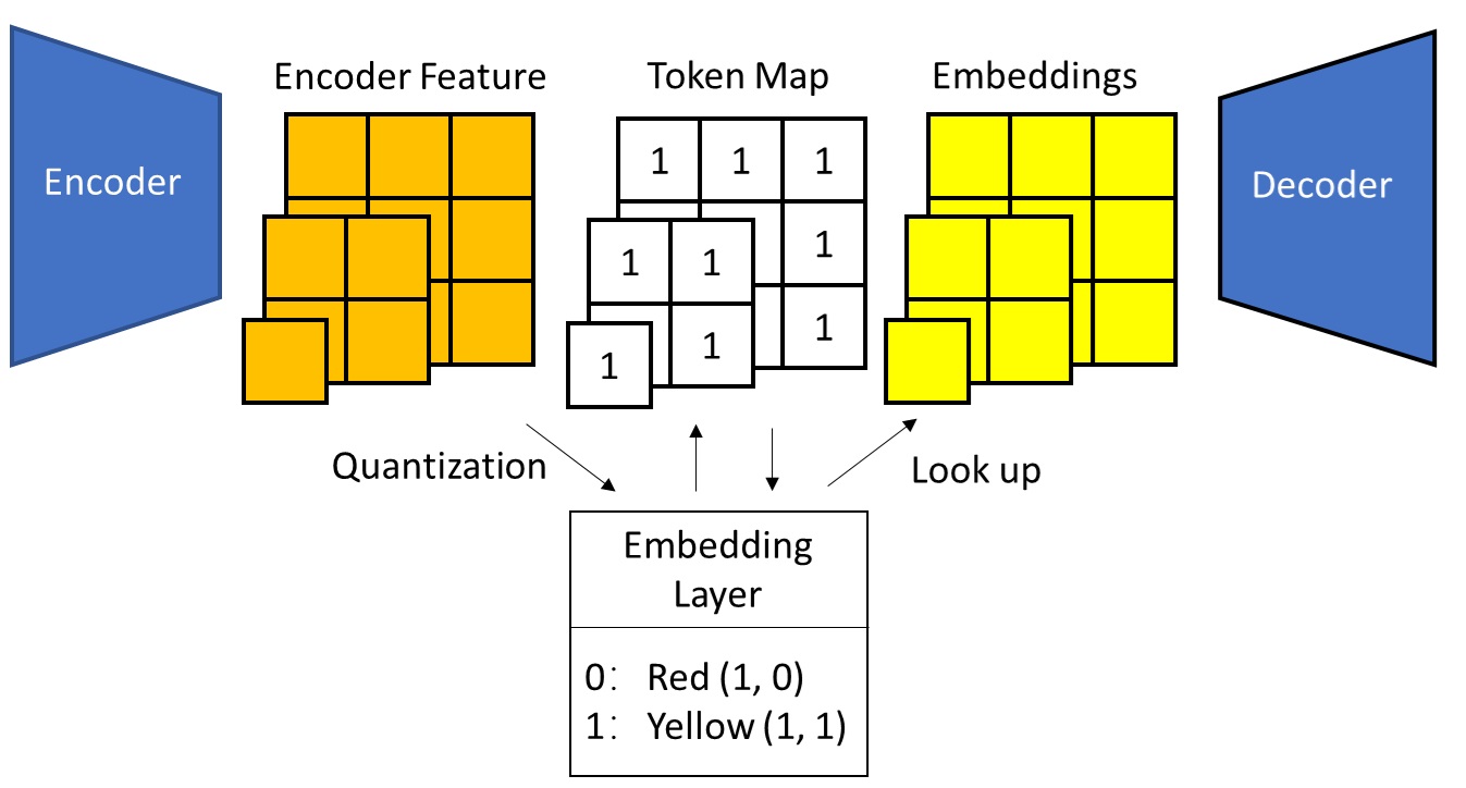
With Block Sparse FlashAttention in mind, an efficient Top-$K$ sparse attention algorithm emerges naturally. The key idea is to construct coarse representations that summarize each block, compute Top-$K$ sparsity on these coarse features, and then apply block-sparse attention. The steps are:

1. Apply $B$-stride average pooling to $\mathbf{Q}$ and $\mathbf{K}$, producing $\mathbf{Q}’, \mathbf{K}’ \in \mathbb{R}^{T \times d}$ with $T = N/B$.
2. Compute inner products between $\mathbf{Q}’$ and $\mathbf{K}’$, and select the Top-$K$ key blocks for each query block.
3. Execute Block Sparse FlashAttention using the resulting sparse block indices.

This description abstracts the core idea behind many modern Top-$K$ sparse attention methods, including MoBA, NSA, and later VMoBA, VSA, and SLA.

Let us analyze the complexity. The runtime is dominated by Top-$K$ search (step 2) and sparse attention computation (step 3).

• Top-$K$ search involves $O((N/B)^2)$ inner products.
• Sparse attention costs $O(NKB)$, since each query attends to $KB$ keys.

When $N$ is small, sparse attention dominates. As $N$ grows, the $O(N^2)$ term inevitably dominates. Thus, such methods do not fundamentally improve attention complexity; they only yield a constant-factor speedup (at most $B^2$). In contrast, the goal of Log-linear Sparse Attention (LLSA) is to eliminate the $O(N^2)$ term entirely.

Related Work

In NLP, popular trainable sparse attention mechanisms include MoBA and NSA. Concurrently, SpargeAttention was proposed as a pooling-and-filtering-based sparse attention applicable to both NLP and CV. In CV, VMoBA adapts MoBA to vision tasks, while VSA (Video Sparse Attention) and SLA (Sparse-Linear Attention) ressolve the information loss caused by sparsity in VMoBA. VSA computes a coarse attention output and adds it to sparse attention, while SLA uses linear attention to approximate contributions from non-Top-$K$ keys.

Hierarchical decompositions with $O(\log N)$ levels are a recurring idea in attention optimization. Early examples include H-Transformer and Fast Multipole Attention. More recently, Radial Attention achieves $O(N\log N)$ complexity via a static sparsity pattern for video. Log-linear Attention improves linear attention quality by maintaining $O(\log N)$ states per query using Fenwick Tree. The method most similar to ours is Multi-Resolution Attention (MRA), which lacks an efficient FlashAttention-compatible GPU implementation and was not validated on ultra-long sequence generation.

LLSA targets Pixel DiT. At the time of this work, Pixel DiT research was limited to PixelFlow and PixNerd. More recently, JiT, DiP, DeCo, and PixelDiT appeared on arXiv, but all rely on patchification to reduce token counts. No prior work trained DiT without VAE and without patchification, due to the prohibitive attention cost. Our work directly addresses this challenge and validates LLSA on high-resolution pure pixel DiT generation.

Log-linear Sparse Attention: Method

The figure below provides an overview of the method.

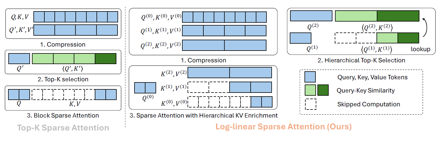
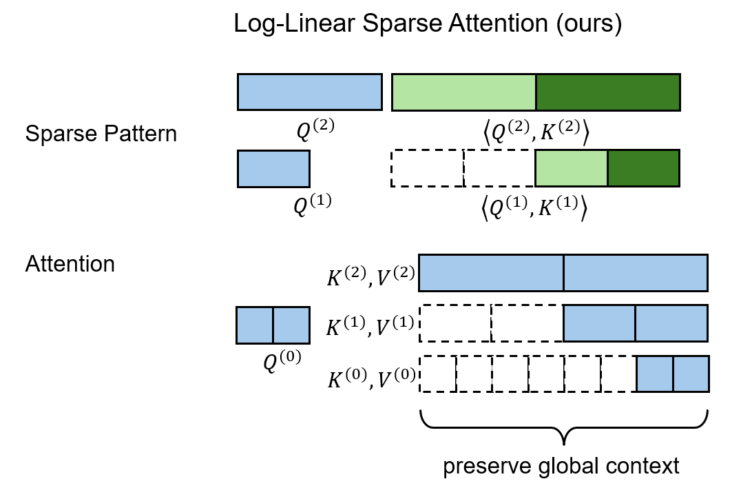
In short, LLSA upgrades the conventional two-level sparsity structure into a multi-level hierarchy. Moreover, in the final sparse attention computation, LLSA not only uses the finest-grained keys/values, but also incorporates coarser keys/values from multiple hierarchy levels. Details are as follows.

Attention Algorithm

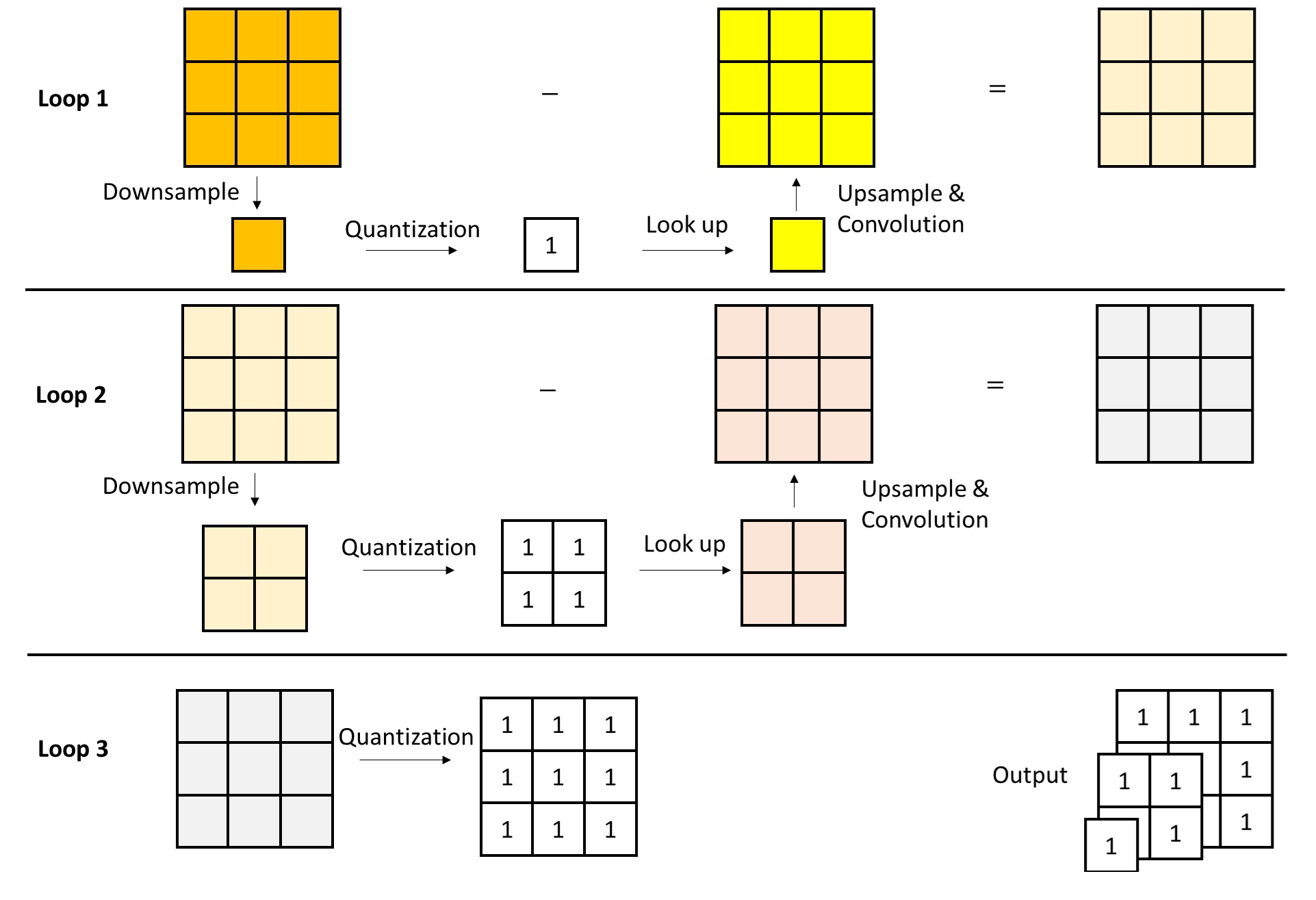
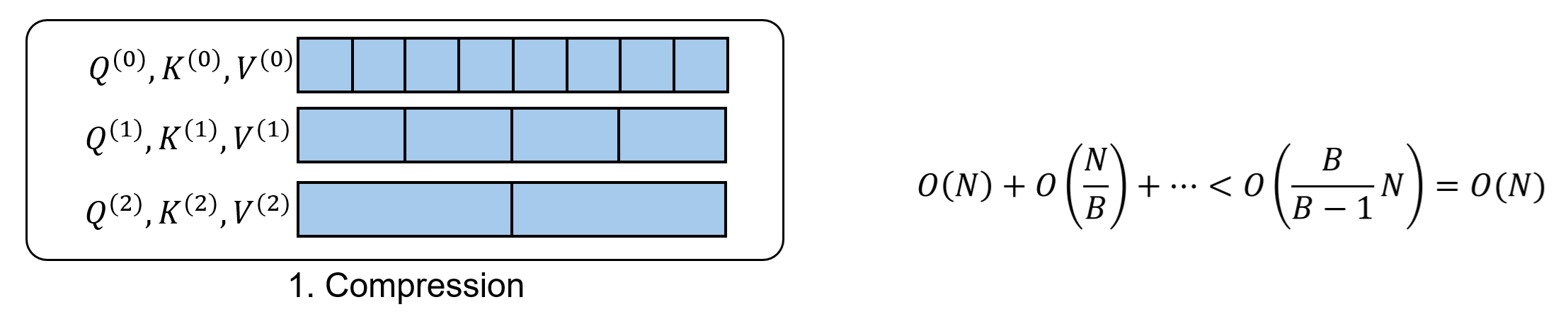
Hierarchical Compression

We partition the token sequence into $
L = \log_B N - 1
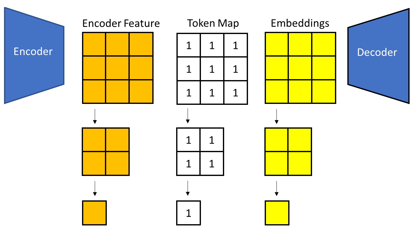
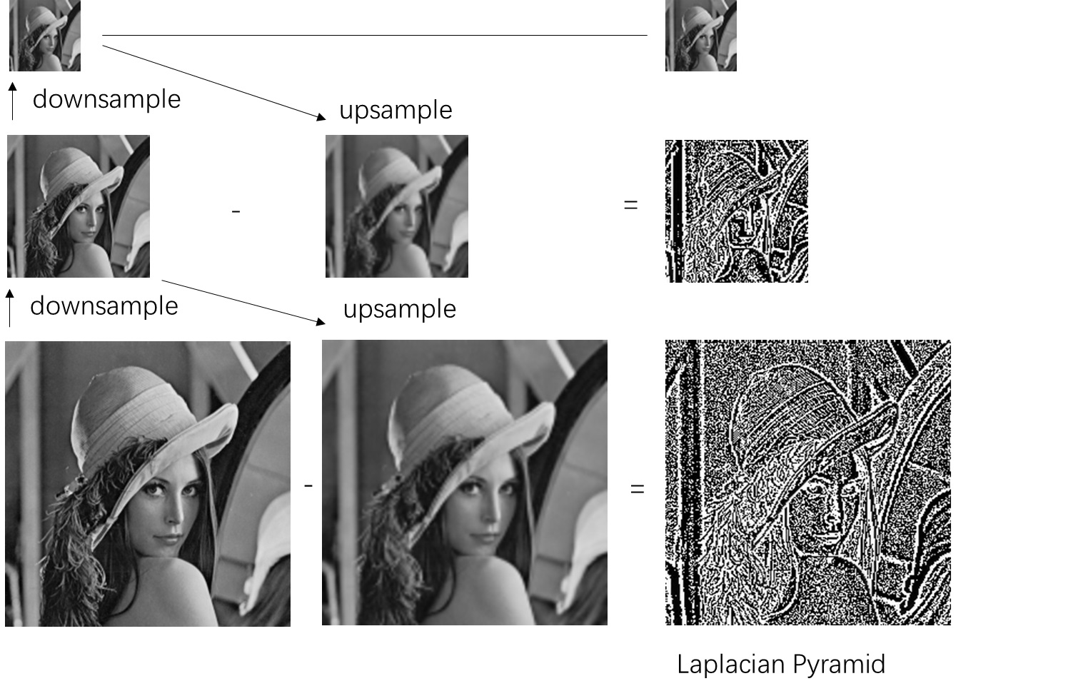
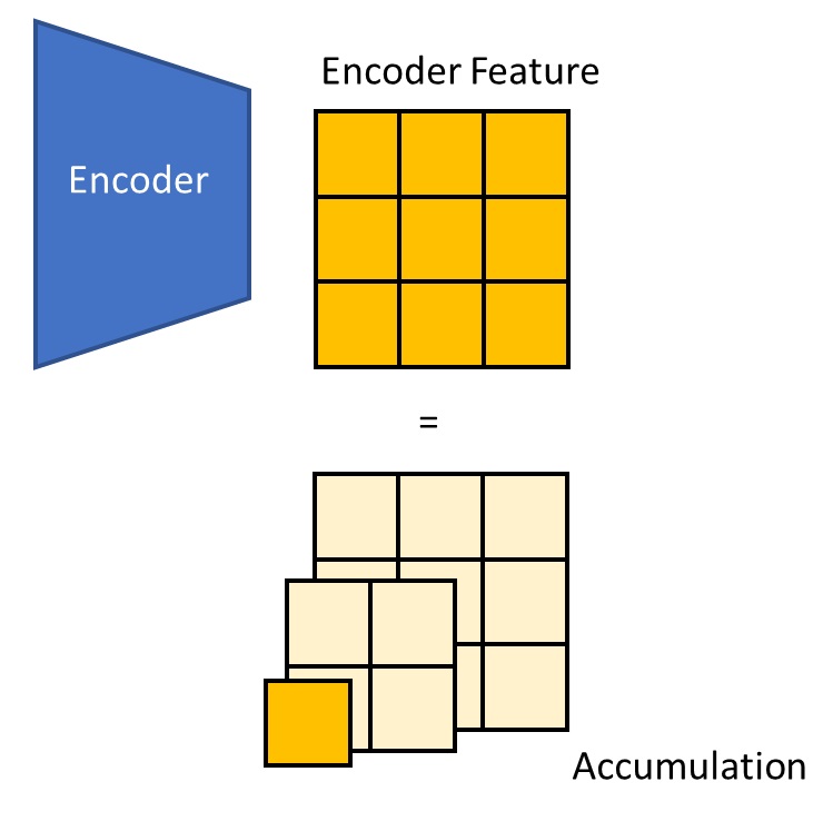
$ levels. Concretely, we repeatedly apply $B$-stride average pooling to compress the original token features

into $L$ sets of coarser tokens. At level $l$, we have

Hierarchical Top-$K$ Selection

We perform Top-$K$ selection in a top-down manner, refining from coarse to fine, to identify the Top-$K$ most similar key blocks for each query block.

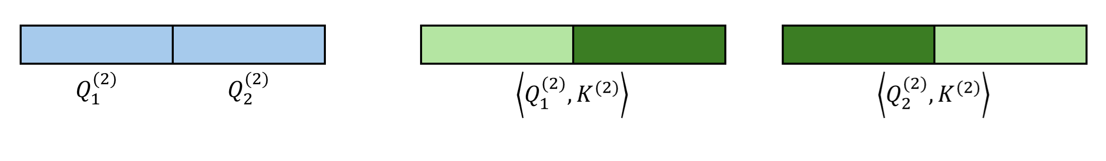
Consider the example $N=8, B=2, K=1$. We start by computing full similarities at the top level (level $L$) between coarse queries and keys.

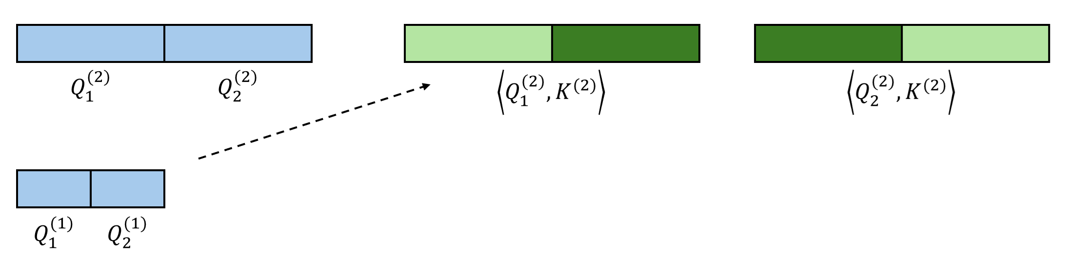
Starting from the second-coarsest level, we recursively leverage the sparse indices from the previous level to further select Top-$K$ candidates. Here, we assume that all fine queries within the same coarse block share the same sparse pattern at this level. For example, in the figure below, both $\mathbf{Q}^{(1)}_1$ and $\mathbf{Q}^{(1)}_2$ belong to the coarser block $\mathbf{Q}^{(2)}_1$, and thus they should only attend to the key tokens corresponding to $\mathbf{K}^{(2)}_2$.

At the previous level, each query has $K$ candidate coarse key blocks. At the current (finer) level, since the granularity increases, each query has $KB$ candidate key blocks. Among these $KB$ candidates, we run Top-$K$ selection again. This recursion continues until the bottom level.

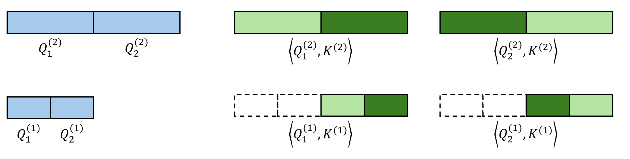
In the end, we obtain the indices of Top-$K$ key blocks for each query block at all levels.

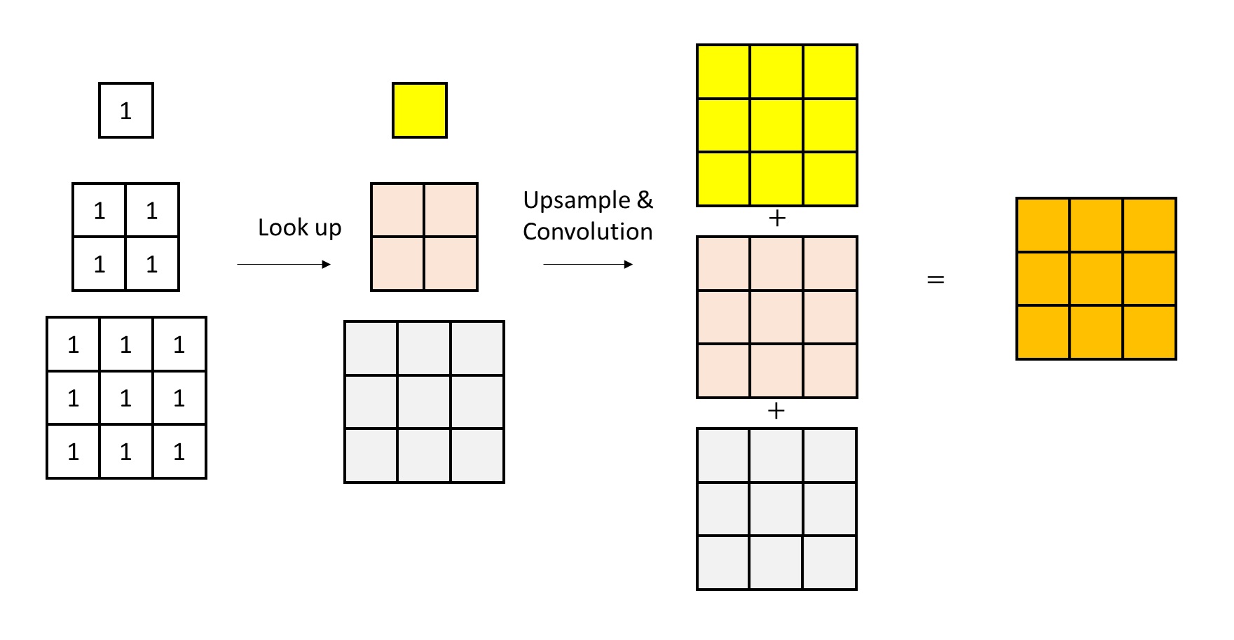
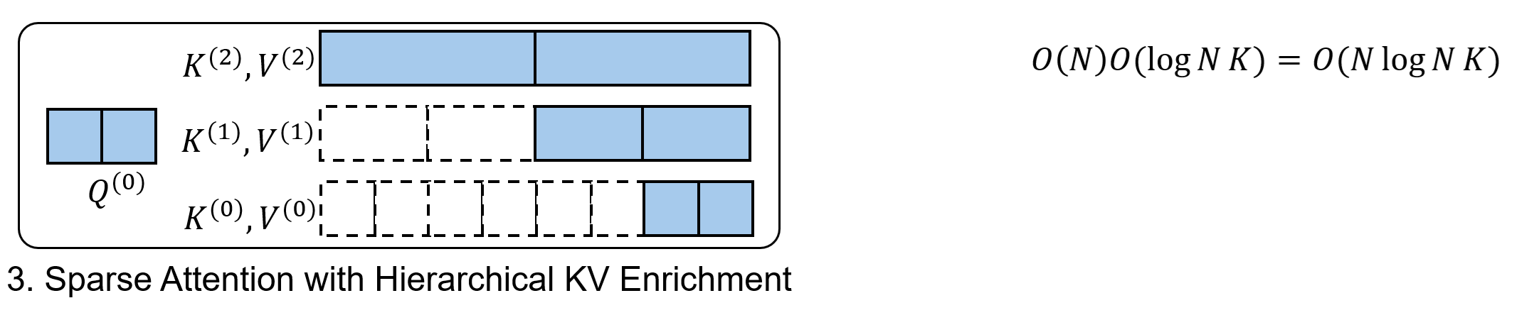
Hierarchical KV Enrichment

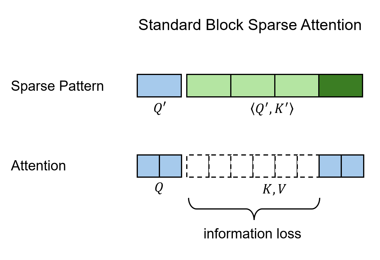
In standard sparse attention, attending only to a sparse subset of K/V tokens inevitably causes information loss.

LLSA mitigates this issue by exploiting the multi-level sparse patterns discovered during hierarchical Top-$K$ selection. Instead of attending only to the finest K/V tokens, LLSA also includes coarser K/V tokens from multiple levels in the final sparse attention computation. This allows each query to preserve global context.

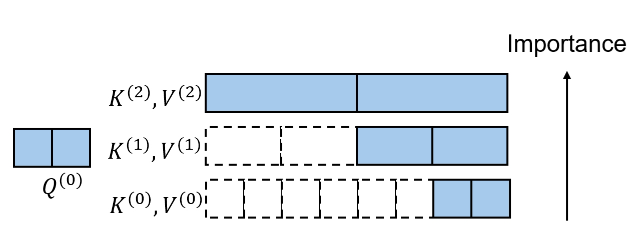
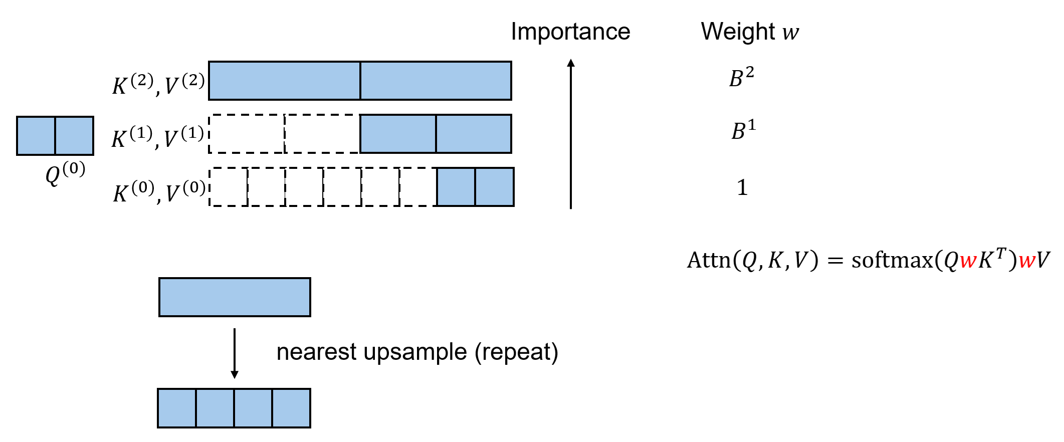
KV Reweighting

The above is not yet optimal. Intuitively, coarser tokens summarize more information and should have higher importance. However, a naive implementation assigns the same weight to K/V tokens from all levels.

We therefore assume that the information in a coarse K/V token can be approximately reconstructed into its fine tokens via nearest-neighbor upsampling (i.e., repeat). Under this assumption, we do not need to explicitly upsample; instead, we can assign different weights to tokens from different levels during attention. Specifically, a level-$l$ token is assigned weight $B^l$, and this weight is applied multiplicatively to both K and V.

Complexity Analysis

Does LLSA truly accelerate prior sparse attention methods? Let us analyze its complexity (assuming $B$ is a constant).

Hierarchical compression. We can count the total number of tokens across levels. Token counts form a geometric series, whose sum is bounded by a constant (dependent on $B$) times $N$. Hence, the complexity is $O(N)$.

Hierarchical Top-$K$ selection. Similarly, the total number of queries across levels is $O(N)$. At each level, the number of candidate key tokens evaluated per query is $KB$, yielding total complexity $O(NK)$.

For simplicity, we do not analyze the complexity of the Top-$K$ algorithm itself. Its complexity depends on the specific implementation, and runtime is tightly coupled with sequence length and the parallel algorithm used. In terms of asymptotic scaling with $N$, when $K$ and $B$ are constants, Top-$K$ selection is also $O(N)$.

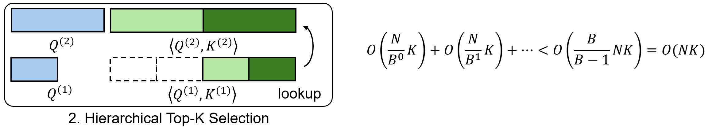
Final attention computation. There are $O(N)$ queries and $O(K\log N)$ key/value blocks per query. Therefore, this step costs $O(NK\log N)$.

If we treat $K$ as a constant as well (which is typical in practice), the overall complexity of LLSA is $O(N\log N)$. In other words, we have reduced the $O(N^2)$ complexity of prior sparse attention mechanisms.

High-Performance GPU Implementation

In modern deep learning frameworks, a new operator must be adapted to GPU parallel programming. LLSA is designed to be compatible with FlashAttention.

Concretely, for all parts involving sparse access (sparse Top-$K$, sparse attention), we can replace dense iteration over all K/V tokens with iteration over sparse indices. We then gather the corresponding K/V values by index. Dense loops that were originally $O(N)$ are reduced to $O(K)$.

However, there is one key challenge in implementation: Top-$K$ selection naturally yields Q-major sparse indices (i.e., which K each Q attends to), but does not directly provide K-major sparse indices (i.e., which Q attends to a given K). Efficient gradient computation for K/V requires K-major indices. Therefore, we must implement a sparse index transpose algorithm that converts Q-major indices into K-major indices.

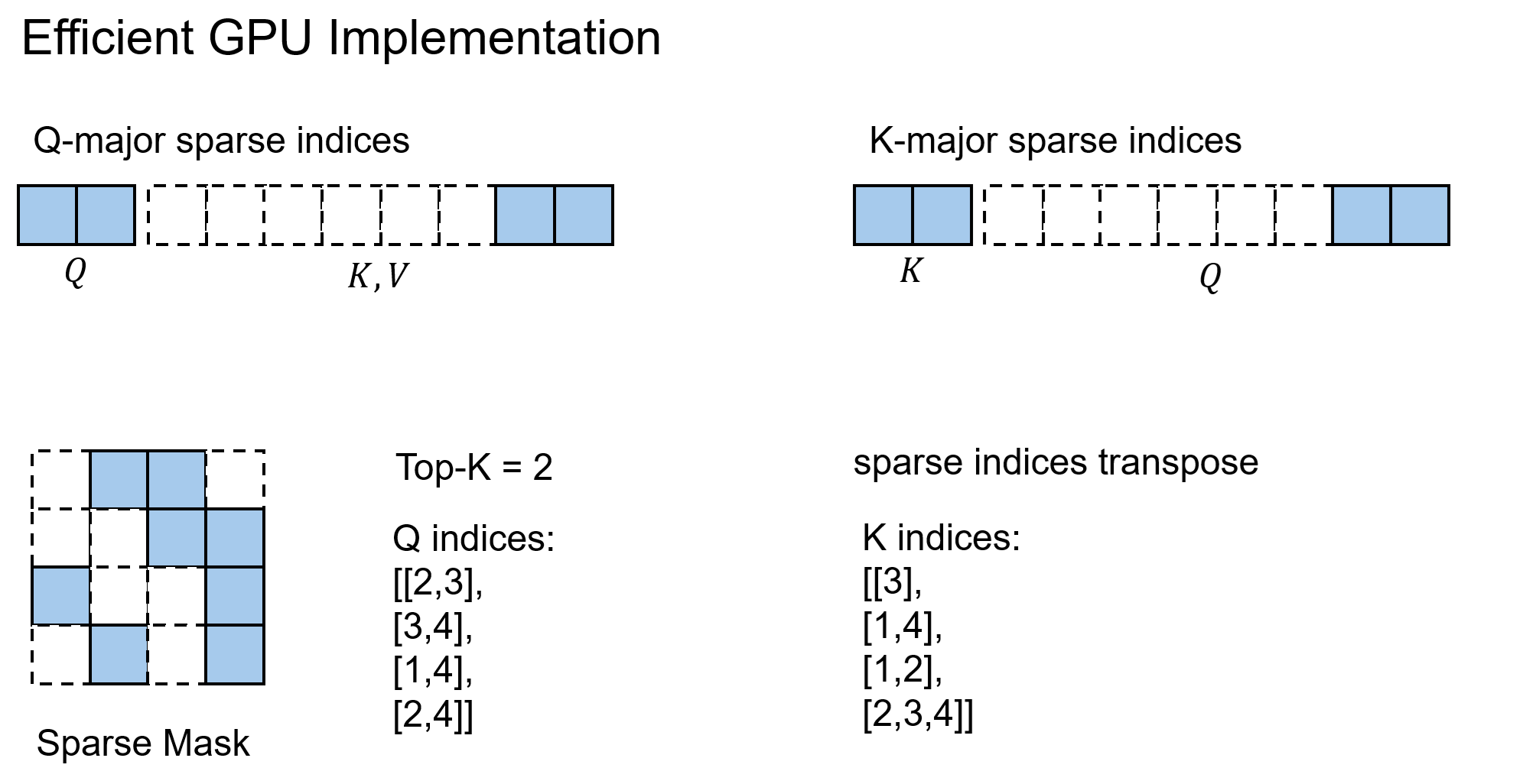
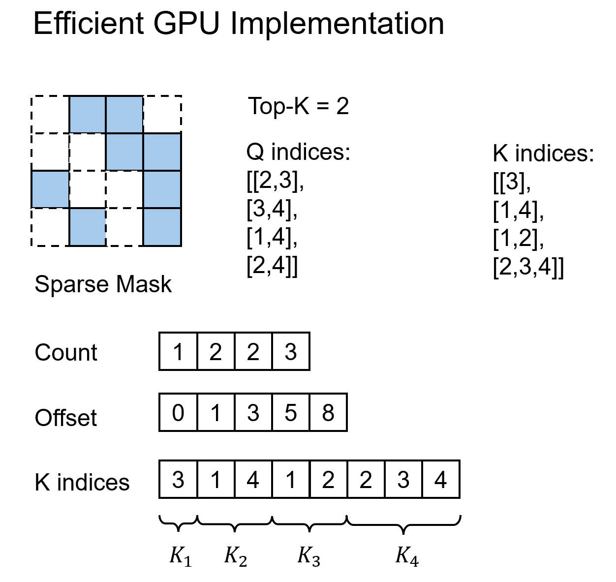
Fortunately, this problem is well studied in sparse matrix multiplication. We directly adopt mature algorithms from that literature. The basic idea is as follows: since the length of K-major indices is variable, we store all K-to-Q indices in a flattened 1D array. This corresponds to flattening a ragged 2D K-major structure. To locate the segment belonging to each K, we maintain an auxiliary offset array that stores the start and end offsets for each K.

Without this optimized approach, one would have to represent sparsity using a dense mask matrix indicating whether each (Q, K) pair is valid. This would degrade complexity back to $O(N^2)$. Many prior methods rely on this less efficient strategy.

Experiments

Pixel DiT Setup

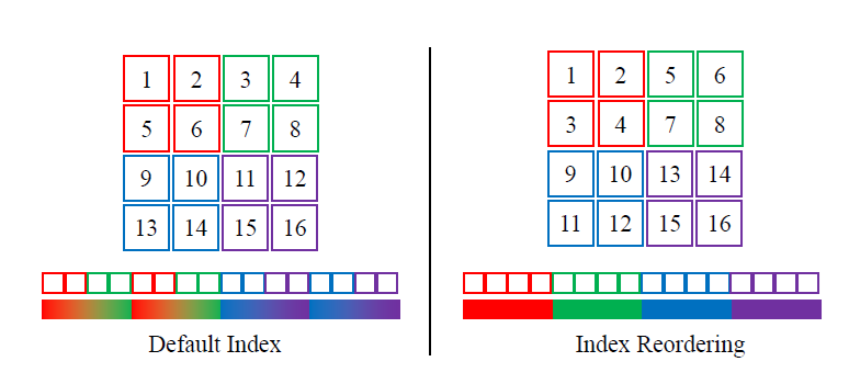
To verify that LLSA indeed reduces the complexity of attention, we train a pure pixel-space DiT without VAE and without patchification on long pixel token sequences. To adapt LLSA to 2D data, we employ index reordering. To accelerate training, we use noise rescaling and low-resolution pretraining.

Index reordering. LLSA is designed for 1D sequences. Since it repeatedly applies average downsampling over adjacent groups of $B$ tokens, it is beneficial if adjacent tokens are semantically correlated. For 2D images, the most natural approach is to map 2D patches into a 1D ordering that preserves locality as much as possible. Following prior work, we adopt the index reordering scheme below.

Noise rescaling. Prior works such as Simple Diffusion and SD3 suggest that higher-resolution data should receive stronger noise. In our experiments, the most effective approach is to multiply the noise term by a factor $s ,(s\ge 1)$. For example, under rectified flow, the noising formula becomes

Empirically, for images of sequence length $n\times n,(n>64)$, we set $
s = \frac{n}{64},
$ i.e., we align the signal-to-noise ratio to that of $64\times 64$ images.

Pretraining. Following multi-stage training strategies used in large-scale text-to-image models such as SD3, we first pretrain on low-resolution images and then progressively finetune at higher resolutions.

DiT architecture. We replace standard DiT positional encoding with RoPE, and add qk-norm to stabilize bfloat16 training.

We do not upgrade the backbone to LightningDiT or DDT, nor do we use REPA.

Metrics. Unless otherwise stated, our default evaluation protocol is: FID is computed on 10,000 samples generated with 20 denoising steps. Throughput is measured in 1,000 pixel tokens per second. All throughput numbers are reported on a single H200 GPU.

Ablations

Unless otherwise specified, ablations are evaluated on models trained for 20 epochs on FFHQ-128. The default hyperparameters are $B=16$ and $K=8$. Key ablation results are shown below.

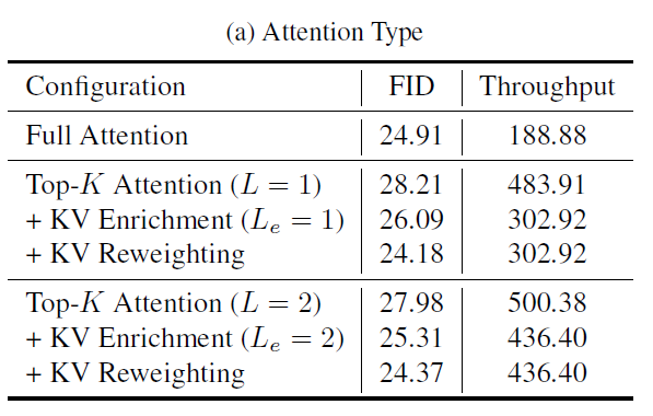
In the table, $L$ denotes the number of hierarchy levels, and $L_e$ denotes how many levels use KV Enrichment. The main takeaways are:

• Comparing $L=1$ vs. $L=2$, moving to $L=2$ significantly improves speed while slightly degrading FID (primarily because the number of KV tokens accessed is greatly reduced). This supports that the $\log N$-level hierarchical design indeed improves computational efficiency.

• Both KV Enrichment and KV Reweighting are effective. In fact, the resulting sparse attention can even outperform full attention in terms of FID.

We also train an $L=3$ LLSA model on FFHQ at $512\times 512$. The outcome matches expectations: as sequence length increases, increasing $L$ yields runtime that grows roughly as $O(N\log N)$. However, since fewer KV tokens are used, speed improves at the cost of slightly worse quality.

The paper and appendix contain more ablation results. Overall, every design choice—both in attention and in training—contributes positively.

Comparisons

We compare LLSA against VSA and SLA, and briefly discuss VMoBA. To my knowledge, these are the three recent works on trainable sparse attention for DiT. If we focus only on which key blocks are used (ignoring image/video handling details), the methods can be summarized as:

• VMoBA: VMoBA (and MoBA) are equivalent to the Top-$K$ attention described earlier.
• VSA: Compute a coarse attention output on pooled Q/K/V, then add it to the sparse attention output.
• SLA: Use an additional linear attention to approximate contributions from keys outside Top-$K$, then add it to the sparse attention output.

To ensure fairness, we re-implement VSA and SLA inside our training environment and match hyperparameters as closely as possible. Since their GPU backward implementations are relatively inefficient, for a fair speed comparison, we upgrade the backward pass of VSA and SLA to a sparse-index-convolution style implementation.

Moreover, because we enable KV Enrichment, for the same $K$, LLSA accesses more K/V tokens during sparse attention. For fairness in quality comparison, we increase $K$ for VSA and SLA so that the number of K/V tokens they actually access matches LLSA’s effective K/V count.

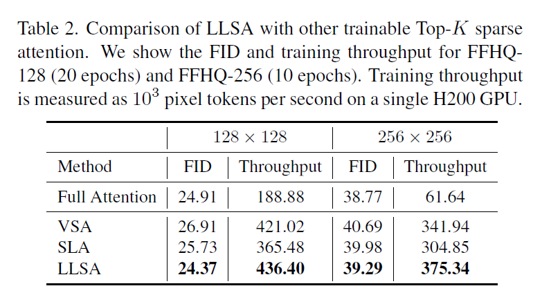
Results on FFHQ are as follows: LLSA is both faster and better.

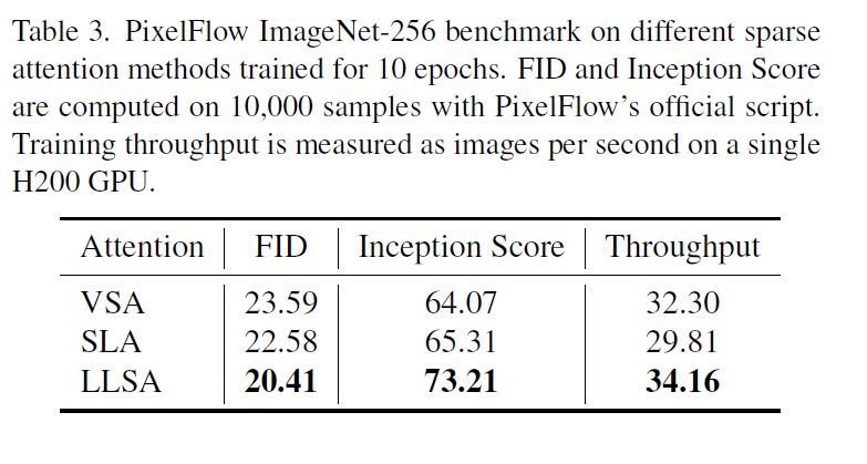
We also run a validation experiment on ImageNet-256. To finish training within limited time, we adopt PixelFlow with patch size = 4 as the DiT backbone, and replace its full attention with VSA, SLA, or LLSA. Results after 10 epochs are shown below.

Metrics during the first four epochs are shown below.

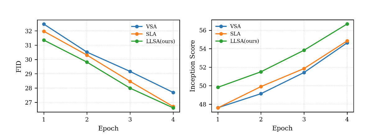
We can see that—even under a conservative experimental setup—LLSA is consistently faster and better than prior sparse attention methods on both FFHQ and ImageNet. This outcome is unsurprising. When designing the attention mechanism, I experimented with many ways of incorporating coarse K/V information. Ultimately, I found that introducing multiple computation branches and summing their outputs (as in VSA/SLA) is consistently inferior to performing a single attention operation that jointly attends to pooled K/V and fine K/V. Thus, even ignoring the $O(\log N)$ acceleration itself, the “coarse+fine K/V in one attention” design improves generation quality compared to prior approaches.

Efficiency

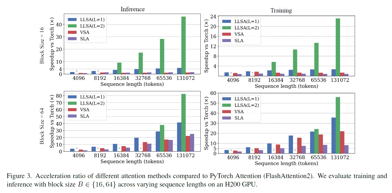
We separately compare inference and training costs (reported as speedup over full attention) across different $B$ values and sequence lengths. Here we use the unoptimized VSA/SLA code. LLSA exhibits a clear efficiency advantage.

We also validate the effectiveness of sparse-index-transpose-based backward. We compare the backward speed of LLSA against a baseline backward that uses a dense sparse mask. Since our algorithm is $O(N)$, throughput remains nearly constant across different sequence lengths.

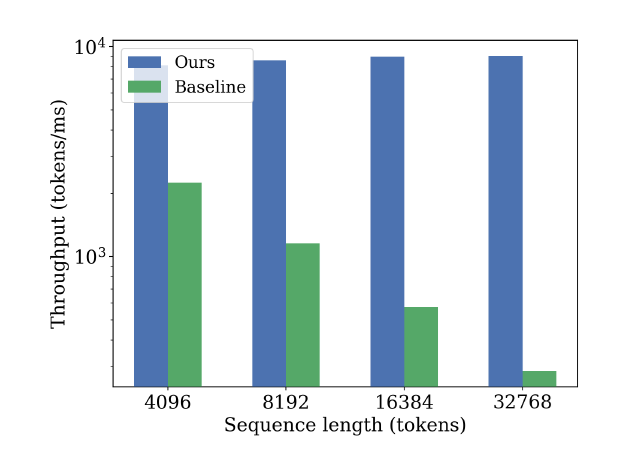
These experiments demonstrate that LLSA also improves upon prior methods in terms of GPU implementation efficiency.

Personal Assessment of the Paper

Based on the experimental results, LLSA consistently outperforms prior methods in terms of efficiency, quality, and GPU implementation. Rather than repeating these results, I will focus on what I consider to be the more interesting limitations of the work.

That said, the paper has two notable weaknesses.

First weakness: One clear limitation of this work is that we do not report fully converged ImageNet-256 results.This is primarily due to the extreme training cost required when attention is applied over full-resolution pixel tokens.

Then why we choose pixel DiT as validation task? Prior methods such as VSA/SLA validate on pretrained video DiTs, where token counts are indeed large and suitable. However, their experimental datasets and evaluation protocols are not very standardized. Furthermore, the VSA paper explicitly states it used 128 GPUs, far beyond what I have access to. Thus, for both fairness and resource reasons, I did not want to choose video generation as the validation task.

High-resolution pure pixel DiT generation is arguably the most fair and clean task for our purpose. Yet even in this setting, the token count is so large that we cannot train as long as DiTs on compressed ImageNet-256 setups. Typically, such DiTs have an effective compression ratio of $16\times 16$. Even under the most optimistic linear scaling assumption, we would need $256\times$ more compute to match their number of training steps. Once we choose “optimize attention complexity” as the goal, it becomes almost inevitable that we cannot afford fully converged training. We therefore settle for comparing methods under limited training budgets.

Second weakness: the paper does not analyze why the hierarchical design is effective. It lacks “theoretical analysis” or strong motivation, and focuses more on implementation details.

This issue is not as severe. Many attention optimization papers primarily present implementation designs. Missing theoretical explanations might lower review scores, but does not invalidate the method. Effectiveness is mainly supported by experiments. If reviewers question this point, we can only acknowledge the limitation.

Finally, there is another point that only attention experts might notice. The method design is extremely similar to Multi-Resolution Attention (MRA), with the key difference that MRA does not provide a high-performance implementation. Does this imply insufficient novelty?

Frankly speaking, when the project started, my goal was to improve upon NSA/VSA-style methods, and I was unaware that an early hierarchical $O(\log N)$ paper already existed. I never believed such an optimization is “unthinkable”—hierarchical algorithmic ideas are common in computer science. However, I do believe that delivering a high-performance GPU implementation is both technically challenging and a substantial contribution. Providing an efficient, ready-to-use implementation likely accounts for more than half of the paper’s value.

Moreover, as discussed earlier, the paper also contributes an algorithmic optimization unrelated to hierarchical attention itself but directly related to sparse attention implementation: the sparse-index-transpose based backward optimization can immediately improve existing VSA/SLA implementations. Overall, I do not think the algorithmic similarity materially undermines the paper’s contribution.

Future Directions

With current resources, my plan is to train a stronger DiT on ImageNet using LLSA. There has been recent work in this direction, such as PixelDiT. I want to see whether we can use LLSA to compute pixel-wise attention somewhere in the model without significantly increasing compute. For example, keep PixelDiT’s patchified encoder unchanged, and only increase attention cost in the decoder. But my recent experiments suggest this does not help much—removing patchification across the entire Transformer seems necessary. For now, I am still exploring low-cost variants.

If we switch validation strategy, another idea is 4K image generation: finetune a pretrained FLUX model on an ultra-high-resolution dataset. Prior work has done similar things but used window attention. Replacing it with LLSA should improve quality substantially. However, such application-driven work requires a much larger engineering effort, and shifts the focus from attention design to a specific task. It is better treated as a separate research project.

In my view, the most efficient path forward is collaboration—validating LLSA on more standard and suitable tasks such as NLP or video DiT generation. For NLP, I would need to connect with researchers working on attention optimization to seek feedback. For video generation, the main bottlenecks are data and compute, so we likely need to collaborate with an industry team. Since the paper studies attention mechanisms themselves, a serious follow-up should not be “small-scale finetuning of existing video models”; ideally, LLSA should be used throughout large-scale training.

Ignoring collaborators and compute constraints entirely, I believe the real stage for LLSA is tasks previously considered infeasible due to quadratic attention, such as voxel-based 3D generation. This year, there is already 3D generation work using sparse attention—for example, Direct3D-S2 adapts NSA to 3D generation and can handle up to 45K 3D latents. If GPU performance continues to improve linearly, and if a task’s quality depends directly on token count, then LLSA should have significant room to shine, because it truly reduces attention complexity.

Summary

In this work, we introduce Log-linear Sparse Attention (LLSA), a novel attention mechanism that reduces self-attention complexity from $O(N^2)$ to $O(N \log N)$. Its main contributions are:

• A hierarchical design that reduces sparse attention complexity, which can be applied to essentially all types of sparse attention mechanisms.

• KV Enrichment, a sparse-attention strategy that better preserves global context than VSA/SLA by attending jointly to sparse fine K/V and coarser K/V tokens.

• A high-performance GPU implementation that we open-source. It can be directly adopted by future work, and its GPU programming insights may also inspire follow-up research.

I see significant potential for LLSA in future large-scale generative models. If I were leading video DiT training, I would immediately replace full attention with LLSA.

My experience in MLSys is still limited, and the paper and research methodology may have room for improvement. We welcome collaboration in various forms, including but not limited to:

• Critiques and suggestions on the paper.
• Academic collaborations with university labs.
• Industry internships or project collaborations.

I will continue to promote and explain the paper. Planned follow-ups include an “exclusive interpretation” blog post beyond the paper content (this post is essentially a restatement of the paper).

References

Attention

(FlashAttention) FlashAttention: Fast and Memory-Efficient Exact Attention with IO-Awareness
(MoBA) MoBA: Mixture of Block Attention for Long-Context LLMs
(NSA) Native Sparse Attention: Hardware-Aligned and Natively Trainable Sparse Attention
(SpargeAttention) SpargeAttention: Accurate and Training-free Sparse Attention Accelerating Any Model Inference
(Sparse VideoGen) Sparse VideoGen: Accelerating Video Diffusion Transformers with Spatial-Temporal Sparsity
(VMoBA) VMoBA: Mixture-of-Block Attention for Video Diffusion Models
(VSA) VSA: Faster Video Diffusion with Trainable Sparse Attention
(SLA) SLA: Beyond Sparsity in Diffusion Transformers via Fine-Tunable Sparse-Linear Attention
(MRA) Multi Resolution Analysis (MRA) for Approximate Self-Attention
(Radial Attention) Radial Attention: $O(n\log n)$ Sparse Attention with Energy Decay for Long Video Generation
Log-Linear Attention

Pixel DiT

(PixelFlow) PixelFlow: Pixel-Space Generative Models with Flow
(PixNerd) PixNerd: Pixel Neural Field Diffusion
(JiT) Back to Basics: Let Denoising Generative Models Denoise
(DiP) DiP: Taming Diffusion Models in Pixel Space
(DeCo) DeCo: Frequency-Decoupled Pixel Diffusion for End-to-End Image Generation
(PixelDiT) PixelDiT: Pixel Diffusion Transformers for Image Generation

Recently, a paper swept through tech media with its eye-catching title: “The GAN is dead; long live the GAN! A Modern Baseline GAN”. I’m not a fan of such extravagant titles—truly valuable research doesn’t need a flashy headline to attract attention. After reading the paper with a hint of resentment, I found that it indeed did not present any particularly significant innovations.

This paper proposes a baseline GAN model called R3GAN (pronounced “Re-GAN”). R3GAN combines the RpGAN loss and a special gradient penalty (GP) loss, and redesigns the GAN architecture based on the state-of-the-art convolutional network ConvNeXt. Experiments show that R3GAN achieves FID scores comparable to those of diffusion models on FFHQ and low-resolution ImageNet image generation. The work mainly contributes through engineering experiments and does not propose many scientific innovations. In this blog post, I will briefly introduce the main implementation details of R3GAN and provide references for each aspect without delving too deeply. Interested readers can refer to the references summarized at the end.

A Review of GANs

In this section, we will review the necessary knowledge related to Generative Adversarial Networks (GANs) that is essential for understanding R3GAN.

Fundamentals of GANs

Like most other generative models, the training objective of a GAN is to model a mapping from an easily sampled distribution (typically a Gaussian distribution) to a distribution that is difficult to train (the training dataset). Specifically, a GAN uses a Generator to transform noise $z$ drawn from a Gaussian distribution into images $x$. While most other generative models have their own theoretical foundations that define the generator’s learning objective, GANs employ another neural network—the Discriminator—to determine the training objective for the generator.

The two models learn via a game: the discriminator attempts to distinguish whether an image is “fake” (i.e., generated) or real, while the generator strives to improve the quality of the generated images so that the discriminator cannot tell the difference. They share the same optimization objective, though one aims to minimize it while the other aims to maximize it.

In the above loss function, there are various choices for the function $f$. R3GAN opts for the softplus function, as illustrated in the figure above.

Two Classic Architectures: DCGAN and StyleGAN

The pioneering GANs were implemented with fully connected networks. In the subsequent development of GANs, two classic architectures emerged: DCGAN in 2016 and StyleGAN in 2019.

DCGAN is a GAN whose generator is based on convolutional neural networks (CNNs). Its hallmark is that it gradually upsamples low-channel features while simultaneously reducing the number of channels, until a three-channel image of the target size is generated.

StyleGAN, on the other hand, is known for its stable training and suitability for image editing. Unlike traditional GAN generators, StyleGAN takes a noise vector $z$ that is preprocessed by a mapping network via a bypass, and injects the information using the AdaIN operation from style transfer. Because the method of inputting the noise changes, the original low-resolution feature map input is replaced by a constant.

Two Major Challenges: Difficult Convergence and Mode Collapse

Compared to other generative models, GANs are often criticized for being “difficult to train”. This difficulty is evident in issues of convergence and mode collapse. Poor convergence implies that the model does not fit the dataset well, and we can use FID to evaluate the similarity between the model’s outputs and the training set. Mode collapse refers to the phenomenon where, for a multi-category dataset, the model generates only a few of the categories, as illustrated below (Image source). To detect mode collapse, we can either have the network randomly generate a large number of images and use another classification network to count the number of categories present, or use the generation recall metric to roughly assess the diversity of the model’s sampling.

R3GAN Implementation

In the introduction, R3GAN criticizes the various small tricks in StyleGAN that are used to enhance GAN stability and advocates for using a generator as simple as possible. Although the paper is written in this manner, R3GAN is in fact based on the earlier DCGAN, with an updated loss function and the incorporation of the latest CNN architectures—making it almost unrelated to the StyleGAN architecture. Let’s examine R3GAN from these two aspects: the loss function and the model architecture.

Loss Function

Regarding the GAN loss that defines the adversarial game, R3GAN replaces the standard GAN loss with the one from the RpGAN (Relativistic Pairing GAN) paper. In contrast, the RpGAN loss feeds the difference between the discriminator outputs for a pair of real and fake samples into the activation function $f$, rather than feeding the outputs separately.

Based on previous research findings, the authors briefly explain the benefits of the RpGAN loss both intuitively and theoretically:

• Traditional GAN losses only require the discriminator to distinguish between real and fake samples, without enforcing that the gap between real and fake samples be as large as possible. By feeding the difference between a pair of real and fake samples into the loss function, the RpGAN loss encourages this gap to be maximized.
• According to theoretical analyses from previous work, under some simple configurations the standard GAN loss can have a number of suboptimal local minima that grow exponentially, whereas every local minimum of the RpGAN loss is a global minimum.

R3GAN also re-examines the optimal gradient penalty (GP) loss through ablation experiments. The term n-GP indicates that the model’s gradient with respect to the input should be as close as possible to the constant $n$, thereby stabilizing training. The commonly used GPs are 0-GP and 1-GP:

• 0-GP: In the optimal case, the model produces exactly the same output for any input.
• 1-GP: In the optimal case, the model’s output changes smoothly with the input; that is, if the norm of the input tensor changes by 1, the norm of the output tensor also changes by 1.

The authors argue that 0-GP is more suitable for the GAN discriminator, because when the generator’s outputs are identical to the training data, the discriminator should be unable to distinguish between any inputs and should give the same output for all.

For applying GP to the discriminator, there are two forms: $R_1$ and $R_2$, which apply the penalty to real and fake data respectively. The authors found that using both $R_1$ and $R_2$ yields better results.

To summarize, R3GAN uses the loss function combination of RpGAN + $R_1$ + $R_2$. The authors demonstrate through simple experiments that this configuration is optimal. As shown in the figure below, on a simple dataset with 1000 categories, the optimal loss configuration is able to generate data for all categories, with a smaller distribution distance $D_{KL}$ (similar to the FID metric—the smaller, the better). Omitting the RpGAN loss results in reduced output diversity and convergence, while omitting $R_2$ causes training to fail completely.

Modernized Convolutional Networks

After identifying a simple yet effective loss function, the R3GAN paper further explores improved convolutional network architectures. The paper mentions five configurations:

• A: The original StyleGAN2.
• B: Removing most of the design elements from StyleGAN2, making the model nearly identical to DCGAN.
• C: Replacing the loss function with the new one discussed in the previous section.
• D: Adding ResNet-style residual connections to the VGG-like network.
• E: Updating ResNet with modules from ConvNeXt.

Let’s skip configuration A and look directly at the differences between configuration B and the early DCGAN. According to the authors, the key differences in configuration B are:

• a) Using the $R_1$ loss.
• b) Employing a smaller learning rate and disabling momentum in the Adam optimizer.
• c) Eliminating normalization layers in all parts of the network.
• d) Replacing transposed convolution with bilinear upsampling.

Notably, if changes a), b), or c) are not implemented, training fails. Item d) is the standard configuration for upsampling in modern neural networks and helps prevent checkerboard artifacts.

The new loss function in configuration C has already been discussed in the previous section.

Prior to this work—including in StyleGAN—most GAN architectures used VGG-like structures without residual blocks. Configuration D introduces the standard 1-3-1 residual blocks from ResNet into the network.

Configuration E further updates the design of the convolutional layers. It first introduces the group convolution operation (dividing channels into groups so that channels within the same group are connected; note that group=1 corresponds to depthwise convolution). Because this operation is more efficient, the network can incorporate more parameters without increasing overall runtime. Additionally, configuration E employs the inverted bottleneck blocks from ConvNeXt, whose design is inspired by the fully connected layers in Transformers.

Let’s review the simple ablation study results for each configuration once more. It appears that the new loss function does not offer much improvement; ultimately, the modifications to the network architecture prove to be more effective. The best configuration, model E, slightly outperforms StyleGAN2.

Quantitative Experimental Results

Finally, let’s examine the quantitative results presented in the paper. As mentioned earlier, we mainly care about two metrics for GANs: diversity and convergence/image quality. The former can be reflected by the number of classes or recall, and the latter can be assessed using FID (and the $D_{KL}$ used in this post).

Diversity

On small multi-class datasets, R3GAN is able to generate all classes and exhibits the best similarity to the training set, whereas StyleGAN2 fails to generate some classes.

Another metric that reflects image diversity is recall, which roughly indicates how much of the training set’s content can be found in the generated set. The paper does not provide detailed tables but merely notes that on CIFAR-10, StyleGAN-XL achieves a recall of 0.47, while R3GAN reaches 0.57. However, overall, R3GAN’s recall is still lower than that of diffusion models.

Convergence

A major highlight touted by this work is that, on certain datasets, its FID scores surpass those of diffusion models. Let’s look at the FID results on both single-class and multi-class datasets.

First, consider the classic FFHQ face dataset. On this dataset, which has relatively low diversity, GANs have generally performed very well. R3GAN achieves a better FID than StyleGAN2 and most diffusion models—and it does so with only a single inference pass (NFE=1). However, its FID does not surpass that of the best previous GAN models. (But those earlier GANs employed a trick to improve FID without enhancing image quality, which R3GAN did not use.)

Next, consider the more diverse CIFAR-10 and ImageNet datasets. R3GAN’s performance is superior to that of all diffusion models and most GANs. However, R3GAN has not been tested on higher-resolution ImageNet. Nowadays, state-of-the-art generative models are typically evaluated on ImageNet-256, but R3GAN does not provide corresponding experimental results.

Summary and Comments

R3GAN is essentially a modernized version of DCGAN. It introduces improvements in two main aspects: the loss function and the model architecture. On the loss function side, DCGAN employs the RpGAN + $R_1$ + $R_2$ loss; on the architecture side, R3GAN replaces the original VGG-like structure with the latest convolutional design from ConvNeXt. Experiments indicate that R3GAN surpasses all diffusion models and most GANs in terms of FID scores on FFHQ-256 and ImageNet-64, although it falls slightly short of the best previous GANs. In terms of generation diversity, however, R3GAN still does not match the performance of diffusion models.

In terms of research contribution, this paper does not introduce any new theories or ideas—it entirely repurposes methods proposed in previous work. Its main contribution lies in offering engineering insights that may help us develop better CNN-based GANs. In terms of experiment results, R3GAN has not been tested on the current mainstream benchmark, ImageNet-256, and there is no evidence that it can outperform diffusion models. From the experimental results on other datasets, one can infer that R3GAN’s best performance is roughly on par with earlier GANs, without making any fundamental improvements to the GAN framework. In summary, I believe this paper is a mediocre work that just meets top conference standards, making its selection as a Poster at NIPS 2024 quite reasonable.

References

• DCGAN: Unsupervised Representation Learning with Deep Convolutional Generative Adversarial Networks
• StyleGAN: A Style-Based Generator Architecture for Generative Adversarial Networks
• StyleGAN2: Analyzing and Improving the Image Quality of StyleGAN
• GP (WGAN-GP): Improved Training of Wasserstein GANs
• RpGAN: The Relativistic Discriminator: A Key Element Missing from Standard GAN
• RpGAN Landscape Explanation: Towards a Better Global Loss Landscape of GANs
• ConvNeXt: A ConvNet for the 2020s
• ImageNet FID Trick: The Role of ImageNet Classes in Fréchet Inception Distance

At the beginning of this year, the multiscale autoregressive model VAR opened a new direction for image generation: by modeling image generation as next-scale prediction, and generating all pixels of the same scale at once per round, VAR achieves high-quality image generation at extremely fast speeds. Subsequently, many works have attempted to improve upon it. To compensate for the information loss introduced by the VQ (Vector Quantization) operation in VAR, HART (Hybrid Autoregressive Transformer) represents the lost information through a residual image and uses a lightweight diffusion model to generate this residual image. With these improvements, the authors used HART to accomplish text-to-image generation at a high resolution of $1024 \times 1024$. In this blog post, we will learn about the core methods of HART and analyze its experimental results on text-to-image tasks.

Paper link: https://arxiv.org/abs/2410.10812

Previous Work

All the autoregressive image generation methods involved in this paper originate from VQVAE and VQGAN. Before reading this paper, it is recommended that readers familiarize themselves with these two classic works.

HART is developed directly based on VAR (Visual Autoregressive Modeling: Scalable Image Generation via Next-Scale Prediction), and some of its ideas are similar to MAR (Masked Autoregressive models, from the paper Autoregressive Image Generation without Vector Quantization). You are welcome to read my previous posts on these.

VAR explaination

On top of the two-stage generation method in VQGAN, VAR makes the encoder output multiple scales of image tokens (instead of only the highest-scale tokens). During generation, VAR autoregressively generates token maps of different scales, and the token map at each scale is generated all at once in a single round of Transformer inference.

The VQ operation causes loss of information in the encoder output, so all image generation models using VQ-based autoencoders end up with slightly reduced quality. Methods like VAR and VQGAN have no choice but to use VQ because they model the distribution of tokens using a categorical distribution. To completely remove VQ, MAR replaces the categorical distribution with a diffusion model, allowing to use a more precise VAE for image compression.

Compensating for VQ’s Information Loss

To mitigate the quality degradation caused by VQ in VAR, HART uses a straightforward approach: since VQ inevitably causes information loss, we can treat that lost information as a residual image. After generating the image with the standard VAR, we use a diffusion model to generate the residual image. Adding the residual image to the original output yields a higher-quality final image.

Let’s get a direct feel for this idea from the figures in the paper. The first row shows reconstruction results from the VAR autoencoder and from HART’s hybrid autoencoder. Due to the VQ operation, the VQ autoencoder struggles to reconstruct the input image. The second row shows the original output from VAR and the residual image. We can see that after adding the residual image, the details become richer, no longer blurry as before.

In the next two sections, we will learn how HART respectively improves the token generation model of VAR and its autoencoder.

Generating Residual Image Using a Diffusion Model

To understand the entire method, we first need to see how HART’s “residual image” comes about. Therefore, let’s look at the modifications on the token generation model, then see the corresponding modifications in the autoencoder.

First, let’s review how VQ errors are introduced in VAR. VAR borrows the classic Laplacian pyramid idea to model token maps at multiple scales.

In other words, VAR does not split the full image into token maps at different resolutions but with the same content. Instead, it splits it into the lowest-resolution image plus the information lost at each scale. This “information loss” includes not only what comes from downsampling but also what results from VQ.

Even though the multiscale decomposition takes into account the information loss from VQ, the final reconstructed features (i.e., the decoder inputs, obtained by summing up the token lookups) still cannot perfectly match the encoder output features. The “residual image” HART wants to generate with a diffusion model is precisely the difference between the reconstructed features and the encoder output features shown in the figure above.

Unlike the discrete token maps, the residual image is continuous. To generate this continuous image, HART refers to MAR, employing an image-conditioned diffusion model. The goal of this diffusion model can be interpreted as: given the decoded image from the discrete token map, how do we use a diffusion model to generate additional details to improve image quality?

A schematic of HART’s generation model is shown below. The generation process before the last step is exactly the same as VAR. In the final step, the intermediate hidden state of the Transformer is fed into an MLP diffusion model. The diffusion model predicts a residual value independently for each token. In other words, this is not an image diffusion model but rather a per-token pixel diffusion model. Tokens are sampled independently from each other. Thanks to this independence assumption, HART can use a lightweight diffusion model to generate the residual image, adding almost no extra time to the overall generation process.

HART also changes VAR’s class conditioning to text conditioning. We will discuss this later in the experiments section.

AE + VQVAE Hybrid Autoencoder

Now that we know where HART’s residual image comes from, we can go back and look at the corresponding modifications in the autoencoder. Currently, the autoencoder decoder has two types of inputs: (1) the approximate reconstructed features formed by summing up the discrete tokens from VAR, and (2) the precise reconstructed features (equal to the encoder output features) when the residual image from HART is added. To handle both types of input simultaneously, the decoder is trained such that half of the time it takes the encoder’s output, and the other half it takes the reconstructed features from the discrete tokens. Of course, during generation, since the residual image is added, the decoder’s input can be considered the same as the encoder output.

The figure below uses “token” terminology differently from VAR. VAR calls both the encoder outputs and decoder inputs “feature maps,” and calls the index map after the VQ operation the “token map.” HART, however, calls the encoder outputs “continuous tokens” and the reconstructed features “discrete tokens”. In this blog post, we follow VAR’s naming. Likewise, what HART calls “residual token” is referred to here as the “residual image.”

In this sense, HART’s hybrid autoencoder is like a VAE without KL loss (i.e., an ordinary autoencoder) and also like a VQVAE.

High-Resolution Text-to-Image Implementation Details

Let’s briefly see how HART extends the class-conditioned ImageNet $256 \times 256$ VAR to a $1024 \times 1024$ text-to-image model.

• Text conditioning: Instead of using cross-attention to incorporate text condition, as in many T2I models, HART follows VAR’s approach to class embeddings, adding the text embedding as the input to the first scale and as input to the AdaLN layers.
• Positional encoding: For the scale and image position indices, VAR uses learnable absolute position embeddings. HART, however, uses sinusoidal encoding for scale and 2D RoPE (rotary position encoding) for the image coordinates.
• Larger scales: In the original VAR, the largest token map side length is 16, HART appends additional side lengths 21,27,36,48,64.
• Lightweight diffusion model: Since the diffusion model only needs to model the distribution of single tokens, it has only 37M parameters and needs just 8 steps to achieve high-quality sampling.

Quantitative Results

• Let’s first look at the most popular “benchmark” metric—ImageNet $256 \times 256$ class-conditioned generation. The authors did not include results for the best MAR model, so I’ve added them here.

In this task, the main difference between HART and VAR is whether or not a diffusion model is used to produce the residual image. As we can see, the residual diffusion model hardly increases the inference time, yet it significantly improves the FID metric (considering the lower the value, the harder it is to improve). Moreover, comparing the speeds of different models, we see that the greatest advantage of VAR-like models lies in their fast inference.

Next, let’s look at the text-to-image generation metrics, which are the main focus of this paper. In addition to the commonly used GenEval (mainly measuring text-image alignment), the authors also show two metrics introduced this year: metrics on the MJHQ-30K dataset and DPG-Bench.

These metrics may not be very convincing. According to user-voted rankings at https://imgsys.org/rankings, Playground v2.5 is the best, while SD3 and PixelArt-Σ are about the same. However, the MJHQ FID and DPG-Bench metrics do not reflect that ranking. In particular, since the FID uses the Inception V3 network trained on ImageNet $299 \times 299$, FID does not accurately capture high-resolution image similarity, nor does it capture similarity in more complex images.

In summary, HART’s performance on high-resolution text-to-image tasks cannot yet be reflected by the experimental results. According to some community feedback (https://www.reddit.com/r/StableDiffusion/comments/1glig4u/mits_hart_fast_texttoimage_model_you_need_to_see/), HART has issues in generating high-frequency details. Looking back at HART’s method, we can infer that this might be caused by the suboptimal design of the residual diffusion model.

Summary

To mitigate the information loss caused by the VQ operation in VQ-based autoencoders, HART treats the lost information as a residual image and uses a lightweight pixel diffusion model to independently generate each pixel of that residual image. HART applies this improvement directly to VAR and boosts the ImageNet FID metric. However, HART still cannot compete with diffusion models in high-resolution text-to-image tasks, and since diffusion models have various acceleration tricks, HART does not have an advantage in generation speed either.

VQ operations transform complex images into image tokens. This makes the distrbution of image tokens easy to learn, but sacrifice autoencoder reconstruction quality. Many works have tried to improve the original nearest-neighbor VQ operation in VQVAE. Regardless, the error introduced by VQ is inevitably present. From another aspect, HART alleviates VQ reconstruction errors by generating a residual image with a separate model. This design idea is promising—it may be possible to eliminate VQ errors entirely. But there’s no free lunch: improving generation quality typically means increasing training and inference time. Although HART’s approach of using a lightweight pixel diffusion model to generate the residual image does not slow down the model, its effectiveness is still not sufficient. Perhaps replacing it with a diffusion model with larger receptive field could improve the quality of the residual image without significantly increasing generation time.

This past April, Peking University (PKU) and ByteDance published a paper on Arxiv titled Visual Autoregressive Modeling: Scalable Image Generation via Next-Scale Prediction, introducing a brand-new paradigm for image generation called Visual Autoregressive Modeling (VAR). This autoregressive generation method represents high-definition images as multi-scale token images and replaces the previously popular next-token prediction with a next-scale prediction approach. On the ImageNet $256×256$ image generation task, VAR outperforms DiT. Our research group was quick to read the paper and found that the work offers notable innovations, though whether it can fully replace diffusion models remains to be seen. Typically, attention on such a paper would gradually decrease over time, but two recent events have catapulted VAR’s popularity to an unprecedented level: serious violations by the paper’s first author resulted in ByteDance suing him for 8 million RMB, and the paper was selected as the best paper at Neurips 2024. Taking this opportunity, I decided to thoroughly study this paper and share my findings.

In this post, I will first review early works closely related to VAR: VQVAE and VQGAN. Then, I will introduce the methodological details and experimental results of the paper, and finally, I will share my own tests and theoretical investigations of the VAR approach. During my reading of the VAR paper, I noticed a design flaw. Experimental results suggest that the paper does not provide a complete analysis of why this approach is effective. I encourage everyone to carefully read that section and share your own insights.

Paper link: https://arxiv.org/abs/2404.02905

Review of VQGAN

VAR can be considered an improved version of VQGAN, which, in turn, builds upon VQVAE. To better understand VAR, the most direct approach is to revisit these two classic works, VQVAE and VQGAN. We will start with the autoregressive generation paradigm, then move on to image autoregressive generation, and finally review the implementation details of VQVAE, VQGAN, and Transformer.

Autoregressive Image Generation

Autoregressive (AR) Generation is a straightforward sequence-generation paradigm: given the first $n$ elements of a sequence, the model outputs the $(n+1)$-th element; we then append the newly generated element to the input sequence and again output the $(n+2)$-th element, and so forth. Below is an example of text autoregressive generation:

1
2
3
4

(empty) -> Thank
Thank   -> you 
you     -> very
very    -> much

Strictly speaking, the model does not output what the next element should be, but rather what it could be, i.e., the probability distribution of the next element. By repeatedly sampling from the distribution of each next element, the model can generate a wide variety of sentences.

AR only applies to sequential data whose order is clearly defined. To use it for images, we need to do two things: 1) break the image into a set of elements, and 2) assign a order number to these elements. The simplest approach is to split the image into pixels and generate them in a left-to-right, top-to-bottom order. For instance, the following is a schematic of the classic image AR model PixelCNN. Suppose the image has $3 \times 3$ pixels, labeled from top-left to bottom-right. When generating the 5th pixel, the model can only use the previously generated 4 pixels. The model outputs a probability distribution for the pixel’s possible grayscale values 0, 1, …, 255.

Incidentally, there are many ways to model probability distributions. Here, we use categorical distribution. The advantage of this is its simplicity and ease of sampling. The downside is that the elements must be discrete values. Even though, theoretically, a pixel’s grayscale value could be any real number between 0 and 1 (assuming it has been normalized), using PixelCNN means we are restricted to 256 discrete values 0, 1/255, 2/255, ..., 1 and cannot represent more precise values.

VQVAE

Although PixelCNN can do image generation, it is extremely slow: since pixels are generated one by one, the rounds of network inference equals to the number of pixels. Is there a way to speed up generation? We hope the size of images we need to generate be smaller.

To accelerate PixelCNN, VQVAE introduced a two-stage image generation method that leverages an image compression network: first generate a compressed image, and then reconstruct it into a realistic image via an image compression network. Because the compressed image contains fewer pixels and it can be reconstructed fast, the entire generation process speeds up considerably.

Below is a generation example using VQVAE. Based on the categorical distribution output by PixelCNN, we can sample a compressed image made up of discrete values. These discrete values are analogous to words in natural language processing (NLP): each discrete value holds a special meaning. We can interpret each discrete value as representing the color of a pixel patch in the original image. By using the image compression network’s decoder, we can reconstruct a clear original image from the compressed image.

The training process for VQVAE is the reverse of the generation process. We start by training an image compression network. This network, composed of an encoder and a decoder, is called an autoencoder. The compressed images are referred to as latent images. Once the autoencoder is trained, we convert all the training images into latent images and train PixelCNN to generate these latent images. Interestingly, only the encoder is used when training PixelCNN, while only the decoder is used at generation time.

In the above discussion, we skipped an implementation detail: how do we make the network handle discrete values as input or output? Inputing discrete values to networks is relatively straightforward: in NLP, we use an embedding layer to convert discrete words into continuous vectors. The approach for inputing disrete values is similar. But how do we get the network to output discrete values? This is where vector quantization (VQ) comes into play.

We are all familiar with quantization—for instance, rounding a decimal to the nearest integer. In essence, rounding is converting a decimal to the nearest integer. By the same logic, for vectors, if we have a predefined set of vectors (analogous to “integers”), vector quantization transforms an arbitrary vector into the nearest known vector, where “nearest” refers to Euclidean distance.

A concrete example is shown below. The encoder outputs some continuous vectors in a 2D featuer map. By searching the nearest-neighbor in the embedding layer (also known as “codebook”), each continuous vector is converted to an integer that represents the index of that nearest neighbor. This index can be treated like a token in NLP, so the encoder’s output features are turned into a token map. Then, when feeding the token map into the decoder, we look up the table (the embedding layer) using those indices to convert the indices back into embedding vectors. Strictly speaking, an autoencoder that compresses images into discrete latent images is called “VQVAE,” but sometimes the term “VQVAE” is used to refer to the entire two-stage generation method.

The terms “encoder features”, “token map”, and “embeddings” have various names in different papers, and most authors only use mathematical symbols to refer to them. Here, we use the terminology from the VAR paper.

We will not dive into the specific learning process of the embedding layer here. If you are not familiar with vector quantization, I recommend carefully studying the original VQVAE paper.

VQGAN

VQVAE’s results are not great, mainly because both its compression network and its generation network are underpowered. Consequently, VQGAN method made improvements on both of VQVAE’s networks:

• VQGAN method replaced the VQVAE with VQGAN (Similar to VQVAE, sometimes we use name of the autoencoder, VQGAN, to denote the entire method). On top of VQVAE, VQGAN adds perceptual loss and a GAN loss during training, which substantially improves the reconstruction quality of the autoencoder.
• Instead of using PixelCNN as the generation model, VQGAN method used a Transformer-based approach.

Transformer

Transformer is currently the most dominant backbone network. Compared with other network architectures, its biggest hallmark is that the elements of a sequence communicate information only through attention operations. To handle the text autoregressive generation task, the earliest Transformers used two special designs:

• Because attention alone cannot reflect the order of input elements, each token embedding is combined with positional encoding before being fed into the network.
• AR requires that earlier tokens not see information from subsequent tokens. Therefore, a mask is added to self-attention to control information flow between tokens.

VQGAN uses the exact same design, treating image tokens like text tokens and generating them with a Transformer.

From Next-Token Prediction to Next-Scale Prediction

Traditional image autoregressive generation employs next-token prediction:

• An autoencoder compresses the image into discrete tokens.
• Tokens are generated one by one in a left-to-right, top-to-bottom order.

Even though the number of tokens is drastically reduced by the autoencoder, generating tokens one at a time is still too slow. To address this, VAR proposes a faster, more intuitive AR strategy:

• An autoencoder compresses the image into multiple scales of discrete token maps. For example, if a single latent image used to be $16 \times 16$, we now represent that same latent image using a series of token maps with scales $1 \times 1, 2 \times 2, …, 16 \times 16$.
• Start from the smallest token map and generate larger token maps in ascending order of scale.

Given this strategy, we must modify both the autoencoder and the generation model. Let us check how VAR accomplishes these modifications.

Multi-Scale Residual Quantization Autoencoder

First, let us look at the changes in the autoencoder. Now, the token maps are not just a single map but multiple maps at different scales. Since the definition of token map has changed, so must the definitions of encoder features and embeddings, as shown below.

We can still use VQVAE’s vector quantization approach. The new question is: how do we merge multiple scales of token maps into a single image, given that the encoder output and the decoder input are each just one image?

The simplest approach is to leave the encoder and decoder unchanged, letting them still take and produce the largest-scale image. Only in the middle (at the vector quantization / embedding lookup stage) do we downsample the image.

VAR, however, uses a more advanced approach: a residual pyramid to represent these latent features. Let us briefly recall the classic Laplacian Pyramid algorithm in image processing. We know that each downsampling step loses some information. If that is the case, we can represent a high-resolution image as a low-resolution image plus its “losses” at each resolution scale. As illustrated below, the rightmost column represents the output of the Laplacian Pyramid.

When computing the Laplacian Pyramid, we repeatedly downsample the image and compute the residual between the current-scale image and the upsampled version of the next-scale image. Then, by upsampling the lowest-resolution image and adding the residuals from each layer, we can accurately reconstruct the high-resolution original image.

Our goal is to do something analogous for the encoder features. How do we split the largest-scale encoder features into a accumulation of different-scale features?

In constructing the Laplacian Pyramid, we rely on two operations: degradation and restoration. For images, degradation is downsampling, and restoration is upsampling. For the latent features output by the encoder, we need to define analogous degradation and restoration. Rather cleverly, instead of simply defining them as downsampling/upsampling, VAR references the paper Autoregressive Image Generation using Residual Quantization, regarding the quantization error introduced by vector quantization as a part of degradation. In other words, our new goal is not to ensure that the sum of all scale features equals the encoder features exactly, but rather that the sum of all scale embeddings is as similar as possible to the encoder features, as depicted below.

Given this, we define degradation as downsampling + vector quantization/embedding lookup, and restoration as upsampling + a learnable convolution. Let us see how VQVAE’s original vector quantization and embedding lookup should be applied in this new context.

First, consider the new multi-scale vector quantization operation. Its input is the encoder features; its output is a series of token maps at different scales. The algorithm starts from the lowest scale, and in each loop outputs the token map at the current scale, then passes the residual features to the input of next scale.

As for the multi-scale embedding lookup operation, its input is the multi-scale token maps, and its output is a single feature image at the largest scale, to be fed into the decoder. For this step, we only need to do an embedding lookup and restoration (upsampling + convolution) on each scale’s token map separately, then sum up the outputs from all scales to get features similar to the encoder’s. Note that for simplicity, these diagrams omit some implementation details, and some numerical values may not be perfectly rigorous.

In summary, to implement scale-wise autoregressive generation, we must encode an image into multi-scale token images. VAR employs a multi-scale residual quantization approach: it decomposes the encoder features into the smallest-scale feature plus residual features at each scale, and applies vector quantization to the features at each scale. This not only effectively split the features into multiple scales but also has another benefit: in standard VQVAE, only the largest-scale features are quantized, making the quantization error large; in VAR, the quantization error is distributed across multiple scales, thereby reducing total quantization error and improving VQVAE’s reconstruction accuracy.

Next-Scale Autoregressive Generation

Once we have compressed the image into multi-scale token maps, the rest is straightforward. We simply flatten all tokens into a one-dimensional sequence and train a Transformer on that sequence. Since the task is now “next-scale prediction,” the model outputs the probability distributions for all tokens at the same scale in one loop, rather than merely the next token. Thus, even though the sequence becomes longer, the model is still faster overall because it can generate all tokens of a given scale in parallel. Meanwhile, the attention masking changes accordingly. Now, tokens at the same scale can see each other, but tokens at previous scales cannot see those at later scales. The following diagram illustrates the difference in attention masks and generation procedures for a
$3 \times 3$ token image under the “next-token” vs. “next-scale” approach.

In addition, the VAR Transformer also includes a few other modifications: 1) besides adding a 1D positional embedding to each token, tokens at the same scale share a scale embedding. All embeddings are learnable; 2) the Transformer and VQVAE decoder share the same embedding layer. Moreover, to reuse information from already generated images when creating a new scale, the initial embeddings for the new scale are obtained by performing bicubic upsampling on the previously generated results.

All other design elements of this Transformer are the same as those in VQGAN. For example, the Transformer has a decoder-only structure, and a special token is used at the first layer to encode the ImageNet class for class-conditional generation. The loss function is cross-entropy loss.

Quantitative Experiments on ImageNet

We have now seen most of the core aspects of VAR’s method. Let us briefly look at its experimental results. The paper claims that VAR performs well in both image generation and model scaling experiments. Specifically, VAR beats DiT in terms of FID score (Fréchet Inception Distance), and its generation speed is more than 45 times faster than DiT. Let us focus on VAR’s results on ImageNet $256 \times 256$ generation task. Below is a table from the paper. I have also included results from the MAR (Autoregressive Image Generation without Vector Quantization) by Kaiming He’s group .

First, let’s compare DiT and VAR. In terms of speed, VAR is clearly much faster than DiT for any model size. In terms of FID as a measure of image quality, for the ~600M parameter regime, DiT still outperforms VAR. However, as the model size increases, DiT’s FID does not show improvement, whereas VAR’s FID keeps dropping. Eventually, VAR’s FID even surpasses that of the ImageNet validation set, at that point, there is little meaning in pushing FID any lower.

Then, let’s compare MAR and VAR. MAR can achieve an even more extreme FID (1.55) with a 943M model. But based on the MAR paper, its speed is about 5 times that of DiT-XL, meaning VAR is still faster—by a factor of around 9 compared to MAR.

On ImageNet, the FID of most SOTA models has essentially been maxed out. The main takeaway from the FID results is that VAR exhibits strong generative capabilities, on par with or better than DiT. However, for more challenging tasks like text-to-image, VAR’s performance is yet to be verified. Moreover, while DiT used 250 sampling steps to produce these benchmark numbers, in practical usage people usually sample in 20 steps. And with distillation, the sampling steps can be reduced to 4. Factoring in these acceleration techniques, VAR might not be faster than DiT.

Visualizing VAR’s Multi-Scale Generation

Having covered the main points of the paper, I will share some of my own theoretical analyses and experimental findings on VAR.

Let us look first at random sampling results. I used the largest VAR model with depth d=30. Under the default settings of the official sampling script, the outputs for two random seeds (0 and 15) are as shown below. The chosen ImageNet classes here are volcano, lighthouse, eagle, and fountain, with two images generated for each class. The generation is very fast, taking only about one second to produce all 8 images.

We can also observe the temporary images decoded at each scale after generation is completed. As expected, the image progresses from coarse to fine detail:

To further investigate which image components each scale is responsible for, we can do the following experiment: from a certain scale onward, switch to a different random seed generator. In GIF of each scale, the unchanged portions come from the earlier scales, and the varying parts come from the subsequent scales. As we can see, from around the third scale onward, the overall content of the image is essentially fixed—that is, structural information is determined in the first two scales. The further we go, the more image details are refined.

These results are rather surprising: does a $2 \times 2$ token map already determine the overall content of the image? Let us examine this in more detail.

Flaws in Single-Scale Generation

Some of you may feel something is off when studying VAR’s sampling algorithm: when generating the token map at a given scale, each token is sampled independently from a probability distribution.

According to the paper, VAR’s scale-autoregressive approach is a new autoregressive probabilistic model:

where $r_k$ denotes the token map at the $k$-th scale (from smallest to largest), and there are $K$ scales in total. Tokens in the same scale $r_k$ are generated in parallel. This means that during training (with a cross-entropy loss) and sampling, the method treats the probability of a token map as the product of the probabilities of all its tokens, assuming independence:

where $r_k^i$ is the $i$-th token at the $k$-th scale, and $I_k$ is the total number of tokens at that scale. I believe the above equation does not hold in principle. Even with the conditions imposed by previous scales, it is unlikely that the distributions for each token in the same scale are mutually independent. And as $I_k$ gets larger, the error introduced by that assumption grows.

Normally, independently sampling tokens at the same scale could result in inconsistencies in the generated image (like a “seam” every 16 pixels if each token represents a
$16 \times 16$ block). But why does VAR’s output still look coherent? On closer inspection of the VAR generation algorithm, we may find two features that greatly reduce discontinuities:

• VAR’s autoencoder uses vector quantization. This ensures the decoder’s input is always “reasonable,” and that the decoded image remains coherent.
• When generating a new scale, the model’s input is initialized with the bicubic upsampling of the previous scale’s image. This bicubic sampling ensures continuity among token embeddings.

Moreover, to further mitigate the negative effects of independent sampling, VAR effectively determines the image’s overall content by the time it completes the second or third scale; subsequent scales only refine image details. (Because as the number of tokens increases, the error from independent sampling grows). We have already verified this through the visualizations above. To show that only the first few scales matter, I did a bold experiment: after the Transformer generates the first two scales of tokens, I randomly generate all subsequent tokens. In the figure below, I froze the outputs of the first two scales and then generated multiple images with different random seeds for the later scales. The results show that if the first two scales are generated well, the rest of the tokens (even if sampled randomly) hardly affect the final image quality.

Based on these experiments, I think the real reason VAR works cannot be merely summarized as “next-scale prediction is a superior new generation paradigm.” The core success factor may be its multi-scale residual quantization autoencoder, which at least accomplishes the following:

• Uses vector quantization to ensure the decoder input is always valid.
• Adopts a multi-scale residual design, where each new scale’s token map not only records the information lost by downsampling but also the precision lost through vector quantization. Compared to a simple, human-interpretable Laplacian pyramid, this learnable degradation process may be more powerful.
• Performs bicubic upsampling of the lower-scale tokens, ensuring continuity in the generated images.

Of course, these components are entangled with one another. Without more in-depth experiments, we cannot pinpoint the single most crucial design element in VAR.

Multi-scale generation itself is not new—prior works like StyleGAN and Cascaded Diffusion have adopted similar strategies. However, VAR makes a bold choice: tokens within the same scale are sampled independently. Surprisingly, this mathematically questionable design does not severely degrade image quality. Thanks to this design, VAR can sample tokens within the same scale in parallel, drastically boosting generation speed.

Conclusions and Commentary

Previously, AR methods like VQGAN fell short in sampling speed and generation quality. The fundamental reasons are that next-token prediction for image tokens is both somewhat misguided and slow. To address this, VAR proposes a new AR strategy: decompose the latent into multiple scales, and generate the latent via next-scale prediction. To accommodate this, VAR modifies both the autoencoder and the Transformer used in VQGAN. In the autoencoder, images are encoded into multi-scale residual token maps, and in the Transformer, each scale’s tokens are assumed to have independent distributions. Experiments show that on ImageNet, VAR surpasses diffusion models like DiT in terms of image quality and is at least 45 times faster. Moreover, experiments suggest that VAR follows the scaling law.

From my perspective, as with other cutting-edge generative models, VAR has essentially maxed out ImageNet FID scores. Its performance on more challenging image-generation tasks remains to be proven. Recently, ByteDance released a text-to-image version of VAR called Infinity, but that model has not been open-sourced yet. We can continue to follow up on subsequent VAR-related work. As for speed, VAR may not be significantly faster than DiT once techniques such as reduced sampling steps and model distillation (for DiT) are applied. Of course, it is possible that VAR can be further accelerated in ways that have not been explored as extensively as with diffusion models.

Mathematically, the VAR approach has flaws: the token map’s distribution should not be the product of the independent distributions of its tokens. At least, the paper does not provide any analysis on this (nor does MAR, which uses a similar approach). Yet, simple generation experiments show that due to other designs that enforce continuity, the model outputs coherent images even if tokens at the same scale are sampled independently or even randomly. We need deeper experiments to really uncover why VAR is so effective.

I think if a research project could clearly explain which parts of VAR are making the biggest difference, retain those and discard the rest to propose a superior generation model, it would be a significant contribution. Potential directions for exploration include:

• Only the first few scales of tokens seem crucial in VAR. Perhaps we could generate those earlier scales using a more refined approach—for instance, a diffusion model—to ensure quality, while using a more efficient (maybe faster than a Transformer) model for the higher-scale token images. This could further enhance both quality and speed.
• VAR still relies on a VQ autoencoder, and no matter how you improve it, vector quantization reduces reconstruction accuracy. On the other hand, VQ can regularize the decoder’s input. Is it possible to replace VQ with VAE for its higher accuracy? And if so, how would we design a multi-scale encoding algorithm without VQ?

Video diffusion models generally have the problem that video quality decreases with the increase of video length. Therefore, the authors of Diffusion Forcing propose a new sequence generation paradigm: Noise of different levels is independently added to each element in the sequence when training sequence diffusion models. The effectiveness of this paradigm is verified by simple video generation and decision-making tasks. I will introduce this work mainly from the perspective of video generation.

Paper arxiv: https://arxiv.org/abs/2407.01392

Previous work

As we will see later, Diffusion Forcing is closely related to the two previous mainstream sequence generation paradigms: autoregressive generation (AR) and full-sequence diffusion models.

In autoregressive sequence generation, the model continually predicts the next (n-th) element based on the first n-1 elements of the sequence. AR is the most common in NLP and is used by both RNN and Transformer.

The diffusion models can directly generate data of any shape. If we treat video not as a sequence of images, but as a “3D image”, we can directly extend a 2D image diffusion model to a 3D video diffusion model. This approach is referred to in this paper as the “full-sequence diffusion model”. Early works using this approach included Video Diffusion Models by the authors of DDPM. The authors of Stable Diffusion also proposed a similar work, Align your Latents: High-Resolution Video Synthesis with Latent Diffusion Models (Video LDM), based on the LDM.

The full-sequence diffusion models can only generate fixed-length video. In order to extend it to long video generation, it has to be combined with AR. However, the quality of frames generated in this method does not match the training set, causing continuous quality degradation in the autoregressive process. Inspired by Cascaded Diffusion Models, Stable Video Diffusion and other works try to mitigate this problem by adding noise to constrained image/video frames.

AR-Diffusion: Auto-Regressive Diffusion Model for Text Generation further explores the combination of AR and full-sequence diffusion models: when generating text with diffusion models, the noise for each token varies, and the earlier the token, the less the noise. Coincidentally, FIFO-Diffusion: Generating Infinite Videos from Text without Training shows how different video frames can be generated with different levels of noise on a pre-trained video diffusion model. Perhaps inspired by these works, Diffusion Forcing systematically explores how to independently add noise to sequence elements during training.

Research Motivation

The author of this paper finds the shortcomings of the AR and full-sequence diffusion models and considers that the two generative paradigms are complementary:

• AR cannot add new optimization objectives in inference time, and there is a quality degradation problem caused by the mismatch of training and inference samples.
• Full-sequence diffusion models cannot generate sequences of varying lengths.

Conversely,

• Full-sequence diffusion models can add Classifier-guidance in inference time and there is only a little degradation within training sequence length.
• AR can generate sequences of varying lengths.

Then, is it possible to combine the two? During sampling, we want the sequence to be generated autoregressively. Meanwhile, from the aspect of noise levels, we hope that each element can be gradually generated from full noise to full clarity. Here is what Diffusion Forcing does: When generating a sequence, the earlier elements have less noise, while the newer elements have more noise. All the elements of different noise levels are denoised at the same time in diffusion models. For example, if the sampling requires 3 DDIM steps and we want to generate 3 frames, a denoising step would make $[x_1^{1/3\cdot T}, x_2^{2/3\cdot T}, x_3^{T}]$ to $[x_1^0, x_2^{1/3\cdot T}, x_3^{2/3\cdot T}]$.

To implement this kind of sampling, we must modify the training approach of diffusion models so that the model can correctly denoise even if the noise levels of inputs are not uniform. Unlike previous works, the authors find that we do not have to fix the noise levels of each element in training as we do in sampling, but can independently sample the noise levels of each frame.

Simple Video Generation Models

The idea of this paper is very concise. Based on the video DDPM, it just changes the noise levels of each frame in training and sampling. To further understand the method of this work, let’s look at the method and experiment of video generation in this paper.

Overall, the training method is the same as the DDPM epsilon-prediction, but with different frame noise levels.

In terms of inter-frame relationships, Diffusion Forcing models causal relationships, meaning that the current frame can only see information from previous frames.

Specifically, this work uses the hidden variables of RNN (exactly GRU) to model the information passed from previous frames. After introducing RNN, the paper complicates the simple formulas of DDPM. I do not recommend readers delve into the contents of the RNN part.

Because of the different noise levels in different frames, we now need to define a two-dimensional noise schedule table for different frames and denoising steps. To create different noise levels at the beginning, the denoising timestep of newer frames will stay in place. The details of the simultaneous denoising algorithm are introduced in the appendix of the paper.

The authors find that Diffusion Forcing can be extended to video generation with infinite length: when generating the next segment, the RNN’s initial hidden state is set to the output of the RNN of the previous segment without a sliding window.

The authors train two baseline models with the same RNN architecture: an autoregressive model and a full-sequence causal diffusion model. The qualitative results show that the results of Diffusion Forcing are better than those of the baseline methods, whether within the training video length or beyond the length. The results can be viewed on the official project website:

https://boyuan.space/diffusion-forcing/

Critical Analysis

At the beginning of the paper, it says that AR lacks the capacity to add conditions in inference. But this is not fatal for video generation, because you can usually add conditions in training and use Classifier-free Guidance in inference.

The authors say they implemented Diffusion Forcing with RNN for simplicity. But it is clear that 3D U-Net should be the easiest and most intuitive way to do this. After all, the earliest video diffusion model was done with 3D U-Net. In the official warehouse, an undergraduate student helped them implement a 3D U-Net with temporal attention that works better than the original video model.

I think the video generation baselines in the paper are not powerful enough. Most autoregressive video generation / image-to-video generation models employ a noise augmentation method proposed in Cascaded Diffusion, which adds noise to the condition image and inputs this noise scale as an additional condition to the denoising model. This design is similar to the Diffusion Forcing’s principle. To illustrate the benefits of the new approach, it is necessary to compare Diffusion Forcing with these more powerful baseline AR models.

The design of the full-sequence video diffusion model looks strange. The motivation of this type of video diffusion model is to treat the video as a 3D image, allowing the exchange of information between frames, and only ensuring the coherence of the video within the training length. The authors now implement a casual version of the full-sequence video model using RNN, which is certainly not as good as the non-casual version. Although the authors say that Diffusion Forcing is always more coherent than the full-sequence diffusion models, I doubt whether Diffusion Forcing can beat non-casual full-sequence diffusion models.

The main benefit of Diffusion Forcing in video generation should be long video generation beyond training length. Therefore, it doesn’t matter if the full-sequence diffusion models perform better within the training length. The author should compare the method that directly combines autoregressive and full-sequence diffusion models to show the superiority of Diffusion Forcing in long video generation.

To sum up, I think the author’s experiment on the video generation task is not sufficient. Indeed, half the paper focuses on decision-making tasks, not just video generation tasks. I believe Diffusion Forcing will mitigate the degradation in long video generation. We may see better long video diffusion models using Diffusion Forcing by large companies. But the fundamental problem with long video generation is the loss of memory, an essential issue that Diffusion Forcing cannot solve.

My biggest inspiration from this work is that we always treat videos as complete 3D data, but forget that video can be treated as an image sequence. If the video is treated as 3D data, different frames can only see the information of other frames at the current denoising time through temporal attention. But for sequential data, we can do more design on the dependence of different frames, such as using different denoising levels like this work. I’ve long been thinking of a sequence-generation paradigm that has a stronger sequence dependency: Can we condition the current element with all information (including intermediate denoising outputs and intermediate variables of the denoising network) from all other elements in all denoising steps? This kind of strongly conditioned sequence model may be helpful to the consistency of multi-view generation and video segment generation. Since the generation is conditioned on another denoising process, any edits we make to this denoising process can naturally propagate to the current element. For example, in video generation, if the entire video is conditioned on the denoising process of the first frame, we can edit the first frame by any image editing method based on the diffusion model and propagate the changes to the whole video. Of course, I just provide a general idea, temporarily without considering the details, you are welcome to think in this direction.

One might also wonder if Diffusion Forcing could be extended to model pixel relationships. I don’t think there’s a problem with training at all. The problem is with inference: Diffusion Forcing needs to predefine the denoising schedule table for different elements and timesteps. For sequential data such as video, it is natural that the earlier the frame, the lower the noise level. However, how to define the denoising schedule of different pixels is not trivial.