This past April, Peking University (PKU) and ByteDance published a paper on Arxiv titled Visual Autoregressive Modeling: Scalable Image Generation via Next-Scale Prediction, introducing a brand-new paradigm for image generation called Visual Autoregressive Modeling (VAR). This autoregressive generation method represents high-definition images as multi-scale token images and replaces the previously popular next-token prediction with a next-scale prediction approach. On the ImageNet $256×256$ image generation task, VAR outperforms DiT. Our research group was quick to read the paper and found that the work offers notable innovations, though whether it can fully replace diffusion models remains to be seen. Typically, attention on such a paper would gradually decrease over time, but two recent events have catapulted VAR’s popularity to an unprecedented level: serious violations by the paper’s first author resulted in ByteDance suing him for 8 million RMB, and the paper was selected as the best paper at Neurips 2024. Taking this opportunity, I decided to thoroughly study this paper and share my findings.
In this post, I will first review early works closely related to VAR: VQVAE and VQGAN. Then, I will introduce the methodological details and experimental results of the paper, and finally, I will share my own tests and theoretical investigations of the VAR approach. During my reading of the VAR paper, I noticed a design flaw. Experimental results suggest that the paper does not provide a complete analysis of why this approach is effective. I encourage everyone to carefully read that section and share your own insights.
Paper link: https://arxiv.org/abs/2404.02905
Review of VQGAN
VAR can be considered an improved version of VQGAN, which, in turn, builds upon VQVAE. To better understand VAR, the most direct approach is to revisit these two classic works, VQVAE and VQGAN. We will start with the autoregressive generation paradigm, then move on to image autoregressive generation, and finally review the implementation details of VQVAE, VQGAN, and Transformer.
Autoregressive Image Generation
Autoregressive (AR) Generation is a straightforward sequence-generation paradigm: given the first $n$ elements of a sequence, the model outputs the $(n+1)$-th element; we then append the newly generated element to the input sequence and again output the $(n+2)$-th element, and so forth. Below is an example of text autoregressive generation:
1 | (empty) -> Thank |
Strictly speaking, the model does not output what the next element should be, but rather what it could be, i.e., the probability distribution of the next element. By repeatedly sampling from the distribution of each next element, the model can generate a wide variety of sentences.

AR only applies to sequential data whose order is clearly defined. To use it for images, we need to do two things: 1) break the image into a set of elements, and 2) assign a order number to these elements. The simplest approach is to split the image into pixels and generate them in a left-to-right, top-to-bottom order. For instance, the following is a schematic of the classic image AR model PixelCNN. Suppose the image has $3 \times 3$ pixels, labeled from top-left to bottom-right. When generating the 5th pixel, the model can only use the previously generated 4 pixels. The model outputs a probability distribution for the pixel’s possible grayscale values 0, 1, …, 255.
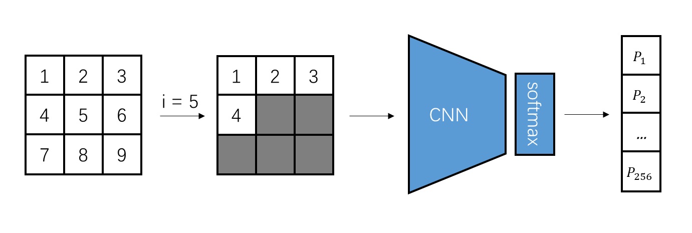
Incidentally, there are many ways to model probability distributions. Here, we use categorical distribution. The advantage of this is its simplicity and ease of sampling. The downside is that the elements must be discrete values. Even though, theoretically, a pixel’s grayscale value could be any real number between 0 and 1 (assuming it has been normalized), using PixelCNN means we are restricted to 256 discrete values 0, 1/255, 2/255, ..., 1 and cannot represent more precise values.
VQVAE
Although PixelCNN can do image generation, it is extremely slow: since pixels are generated one by one, the rounds of network inference equals to the number of pixels. Is there a way to speed up generation? We hope the size of images we need to generate be smaller.
To accelerate PixelCNN, VQVAE introduced a two-stage image generation method that leverages an image compression network: first generate a compressed image, and then reconstruct it into a realistic image via an image compression network. Because the compressed image contains fewer pixels and it can be reconstructed fast, the entire generation process speeds up considerably.
Below is a generation example using VQVAE. Based on the categorical distribution output by PixelCNN, we can sample a compressed image made up of discrete values. These discrete values are analogous to words in natural language processing (NLP): each discrete value holds a special meaning. We can interpret each discrete value as representing the color of a pixel patch in the original image. By using the image compression network’s decoder, we can reconstruct a clear original image from the compressed image.
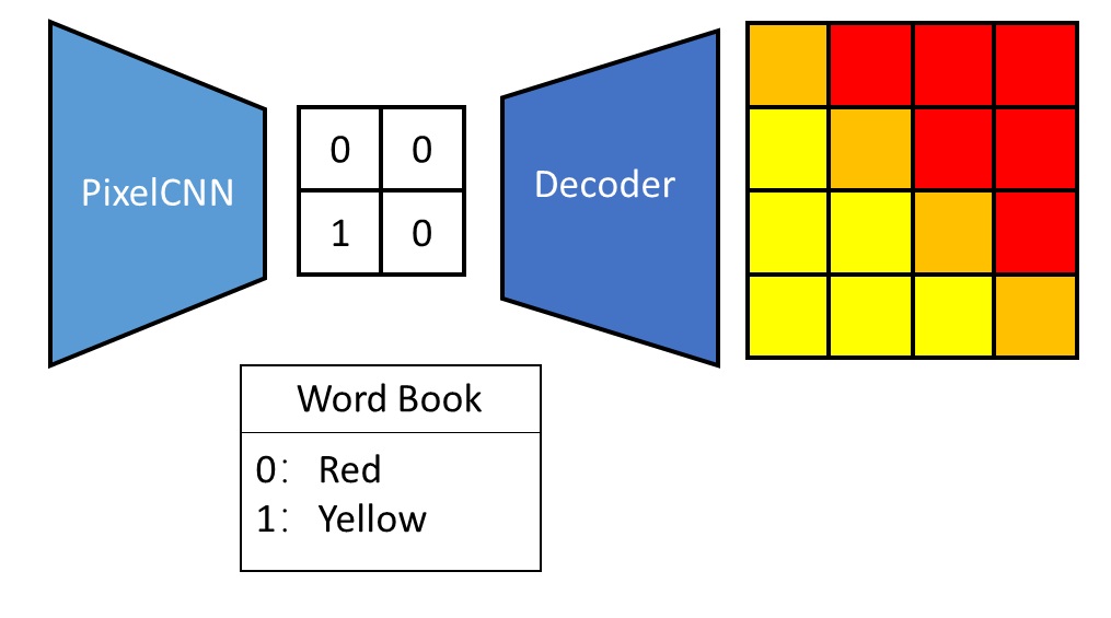
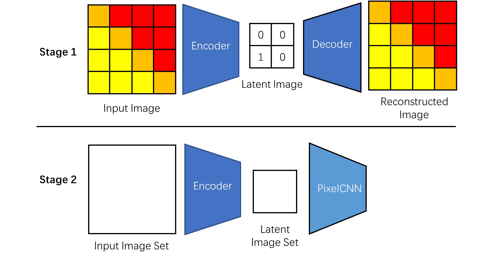
The training process for VQVAE is the reverse of the generation process. We start by training an image compression network. This network, composed of an encoder and a decoder, is called an autoencoder. The compressed images are referred to as latent images. Once the autoencoder is trained, we convert all the training images into latent images and train PixelCNN to generate these latent images. Interestingly, only the encoder is used when training PixelCNN, while only the decoder is used at generation time.
In the above discussion, we skipped an implementation detail: how do we make the network handle discrete values as input or output? Inputing discrete values to networks is relatively straightforward: in NLP, we use an embedding layer to convert discrete words into continuous vectors. The approach for inputing disrete values is similar. But how do we get the network to output discrete values? This is where vector quantization (VQ) comes into play.
We are all familiar with quantization—for instance, rounding a decimal to the nearest integer. In essence, rounding is converting a decimal to the nearest integer. By the same logic, for vectors, if we have a predefined set of vectors (analogous to “integers”), vector quantization transforms an arbitrary vector into the nearest known vector, where “nearest” refers to Euclidean distance.
A concrete example is shown below. The encoder outputs some continuous vectors in a 2D featuer map. By searching the nearest-neighbor in the embedding layer (also known as “codebook”), each continuous vector is converted to an integer that represents the index of that nearest neighbor. This index can be treated like a token in NLP, so the encoder’s output features are turned into a token map. Then, when feeding the token map into the decoder, we look up the table (the embedding layer) using those indices to convert the indices back into embedding vectors. Strictly speaking, an autoencoder that compresses images into discrete latent images is called “VQVAE,” but sometimes the term “VQVAE” is used to refer to the entire two-stage generation method.
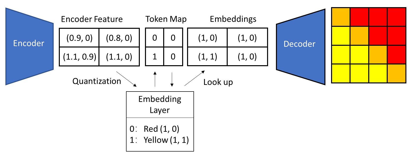
The terms “encoder features”, “token map”, and “embeddings” have various names in different papers, and most authors only use mathematical symbols to refer to them. Here, we use the terminology from the VAR paper.
We will not dive into the specific learning process of the embedding layer here. If you are not familiar with vector quantization, I recommend carefully studying the original VQVAE paper.
VQGAN
VQVAE’s results are not great, mainly because both its compression network and its generation network are underpowered. Consequently, VQGAN method made improvements on both of VQVAE’s networks:
- VQGAN method replaced the VQVAE with VQGAN (Similar to VQVAE, sometimes we use name of the autoencoder, VQGAN, to denote the entire method). On top of VQVAE, VQGAN adds perceptual loss and a GAN loss during training, which substantially improves the reconstruction quality of the autoencoder.
- Instead of using PixelCNN as the generation model, VQGAN method used a Transformer-based approach.
Transformer
Transformer is currently the most dominant backbone network. Compared with other network architectures, its biggest hallmark is that the elements of a sequence communicate information only through attention operations. To handle the text autoregressive generation task, the earliest Transformers used two special designs:
- Because attention alone cannot reflect the order of input elements, each token embedding is combined with positional encoding before being fed into the network.
- AR requires that earlier tokens not see information from subsequent tokens. Therefore, a mask is added to self-attention to control information flow between tokens.
VQGAN uses the exact same design, treating image tokens like text tokens and generating them with a Transformer.
From Next-Token Prediction to Next-Scale Prediction
Traditional image autoregressive generation employs next-token prediction:
- An autoencoder compresses the image into discrete tokens.
- Tokens are generated one by one in a left-to-right, top-to-bottom order.
Even though the number of tokens is drastically reduced by the autoencoder, generating tokens one at a time is still too slow. To address this, VAR proposes a faster, more intuitive AR strategy:
- An autoencoder compresses the image into multiple scales of discrete token maps. For example, if a single latent image used to be $16 \times 16$, we now represent that same latent image using a series of token maps with scales $1 \times 1, 2 \times 2, …, 16 \times 16$.
- Start from the smallest token map and generate larger token maps in ascending order of scale.
Given this strategy, we must modify both the autoencoder and the generation model. Let us check how VAR accomplishes these modifications.
Multi-Scale Residual Quantization Autoencoder
First, let us look at the changes in the autoencoder. Now, the token maps are not just a single map but multiple maps at different scales. Since the definition of token map has changed, so must the definitions of encoder features and embeddings, as shown below.
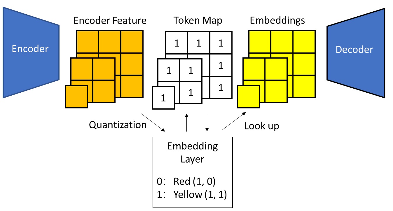
We can still use VQVAE’s vector quantization approach. The new question is: how do we merge multiple scales of token maps into a single image, given that the encoder output and the decoder input are each just one image?
The simplest approach is to leave the encoder and decoder unchanged, letting them still take and produce the largest-scale image. Only in the middle (at the vector quantization / embedding lookup stage) do we downsample the image.
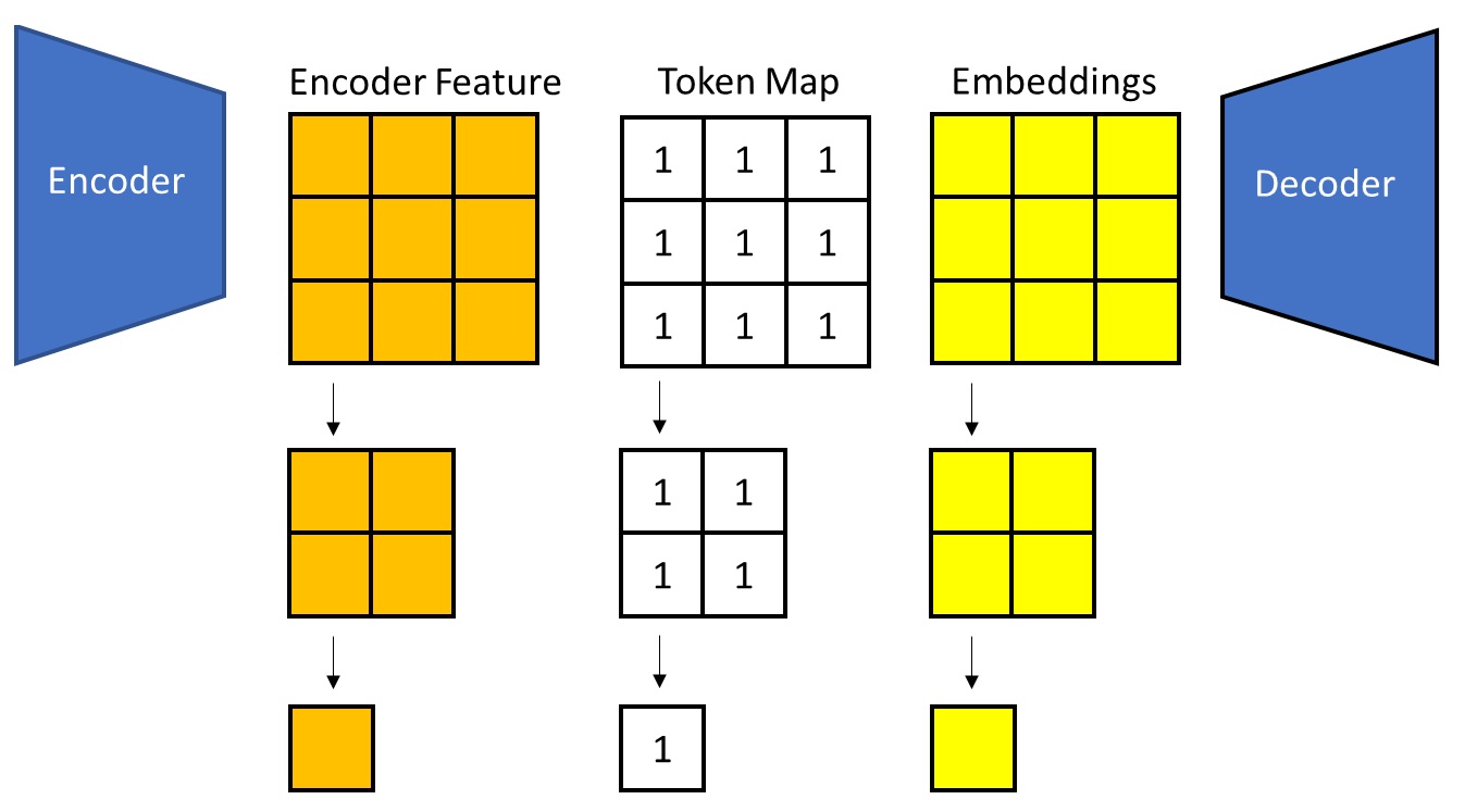
VAR, however, uses a more advanced approach: a residual pyramid to represent these latent features. Let us briefly recall the classic Laplacian Pyramid algorithm in image processing. We know that each downsampling step loses some information. If that is the case, we can represent a high-resolution image as a low-resolution image plus its “losses” at each resolution scale. As illustrated below, the rightmost column represents the output of the Laplacian Pyramid.
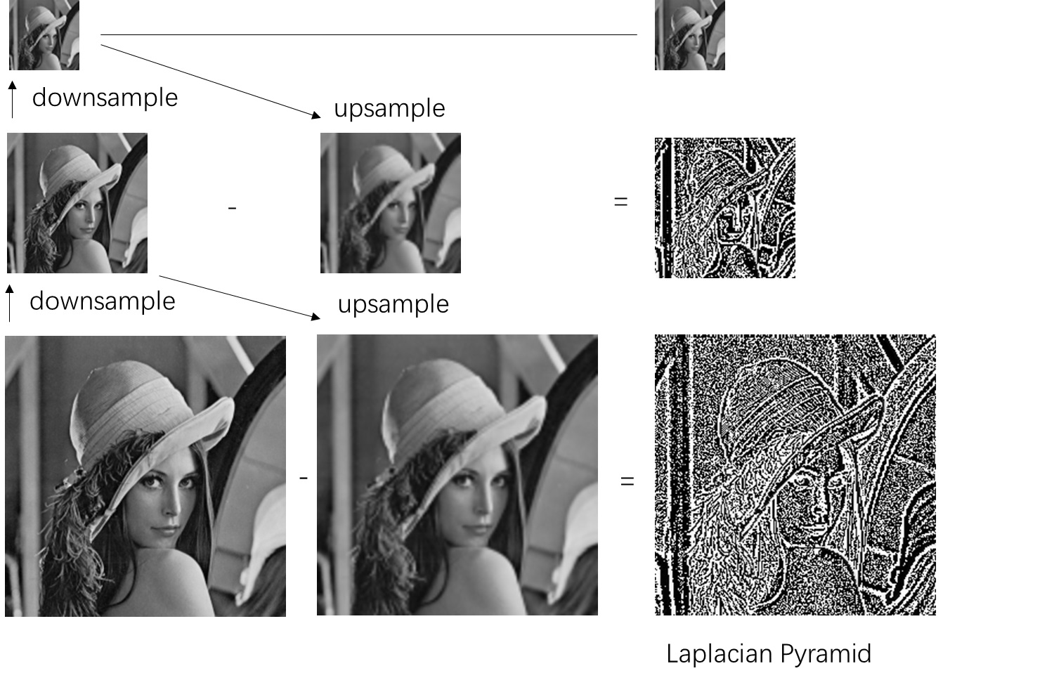
When computing the Laplacian Pyramid, we repeatedly downsample the image and compute the residual between the current-scale image and the upsampled version of the next-scale image. Then, by upsampling the lowest-resolution image and adding the residuals from each layer, we can accurately reconstruct the high-resolution original image.
Our goal is to do something analogous for the encoder features. How do we split the largest-scale encoder features into a accumulation of different-scale features?
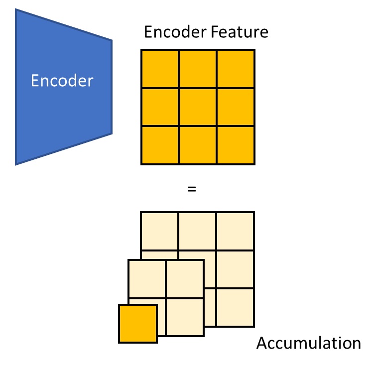
In constructing the Laplacian Pyramid, we rely on two operations: degradation and restoration. For images, degradation is downsampling, and restoration is upsampling. For the latent features output by the encoder, we need to define analogous degradation and restoration. Rather cleverly, instead of simply defining them as downsampling/upsampling, VAR references the paper Autoregressive Image Generation using Residual Quantization, regarding the quantization error introduced by vector quantization as a part of degradation. In other words, our new goal is not to ensure that the sum of all scale features equals the encoder features exactly, but rather that the sum of all scale embeddings is as similar as possible to the encoder features, as depicted below.
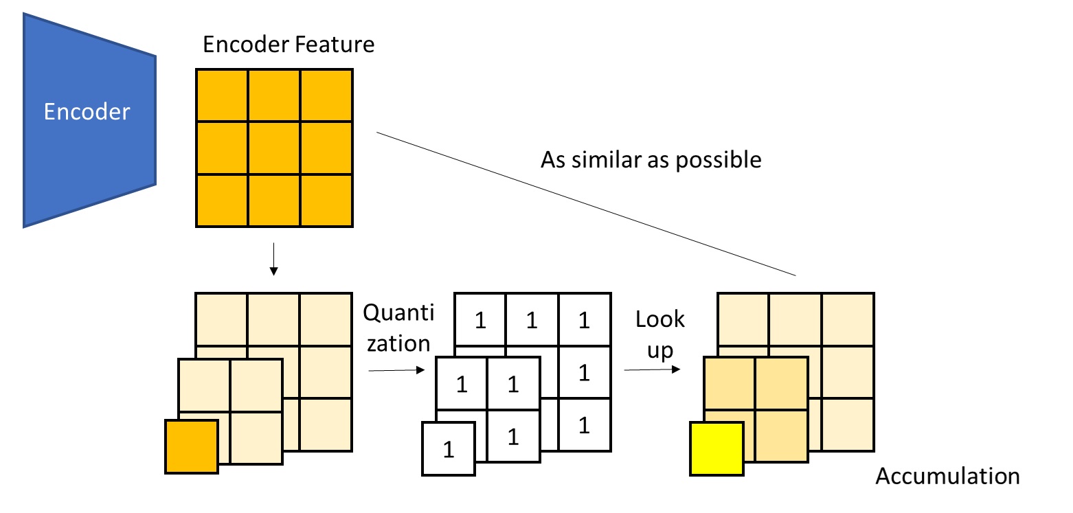
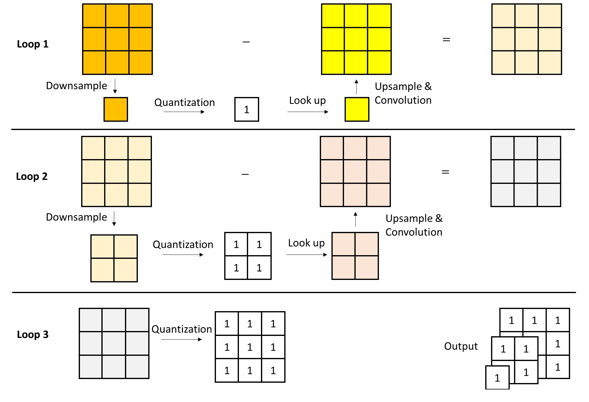
Given this, we define degradation as downsampling + vector quantization/embedding lookup, and restoration as upsampling + a learnable convolution. Let us see how VQVAE’s original vector quantization and embedding lookup should be applied in this new context.
First, consider the new multi-scale vector quantization operation. Its input is the encoder features; its output is a series of token maps at different scales. The algorithm starts from the lowest scale, and in each loop outputs the token map at the current scale, then passes the residual features to the input of next scale.
As for the multi-scale embedding lookup operation, its input is the multi-scale token maps, and its output is a single feature image at the largest scale, to be fed into the decoder. For this step, we only need to do an embedding lookup and restoration (upsampling + convolution) on each scale’s token map separately, then sum up the outputs from all scales to get features similar to the encoder’s. Note that for simplicity, these diagrams omit some implementation details, and some numerical values may not be perfectly rigorous.
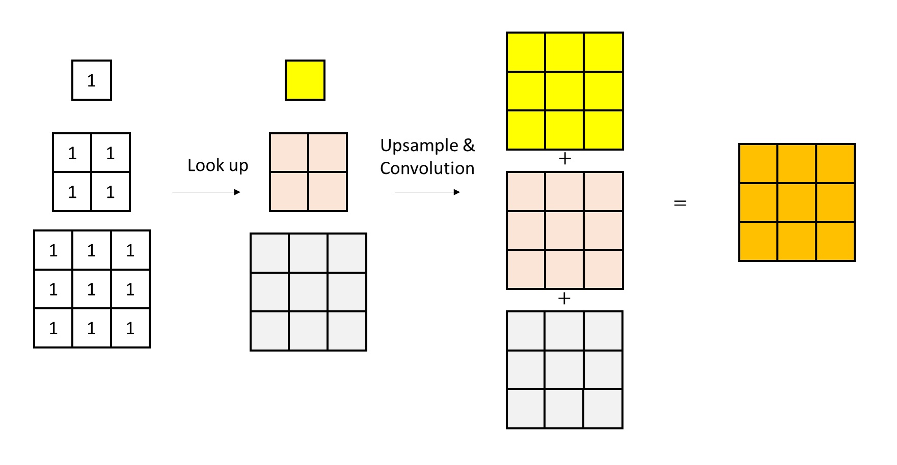
In summary, to implement scale-wise autoregressive generation, we must encode an image into multi-scale token images. VAR employs a multi-scale residual quantization approach: it decomposes the encoder features into the smallest-scale feature plus residual features at each scale, and applies vector quantization to the features at each scale. This not only effectively split the features into multiple scales but also has another benefit: in standard VQVAE, only the largest-scale features are quantized, making the quantization error large; in VAR, the quantization error is distributed across multiple scales, thereby reducing total quantization error and improving VQVAE’s reconstruction accuracy.
Next-Scale Autoregressive Generation
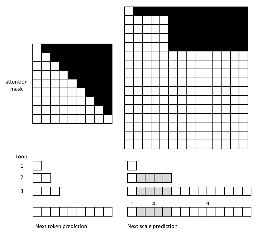
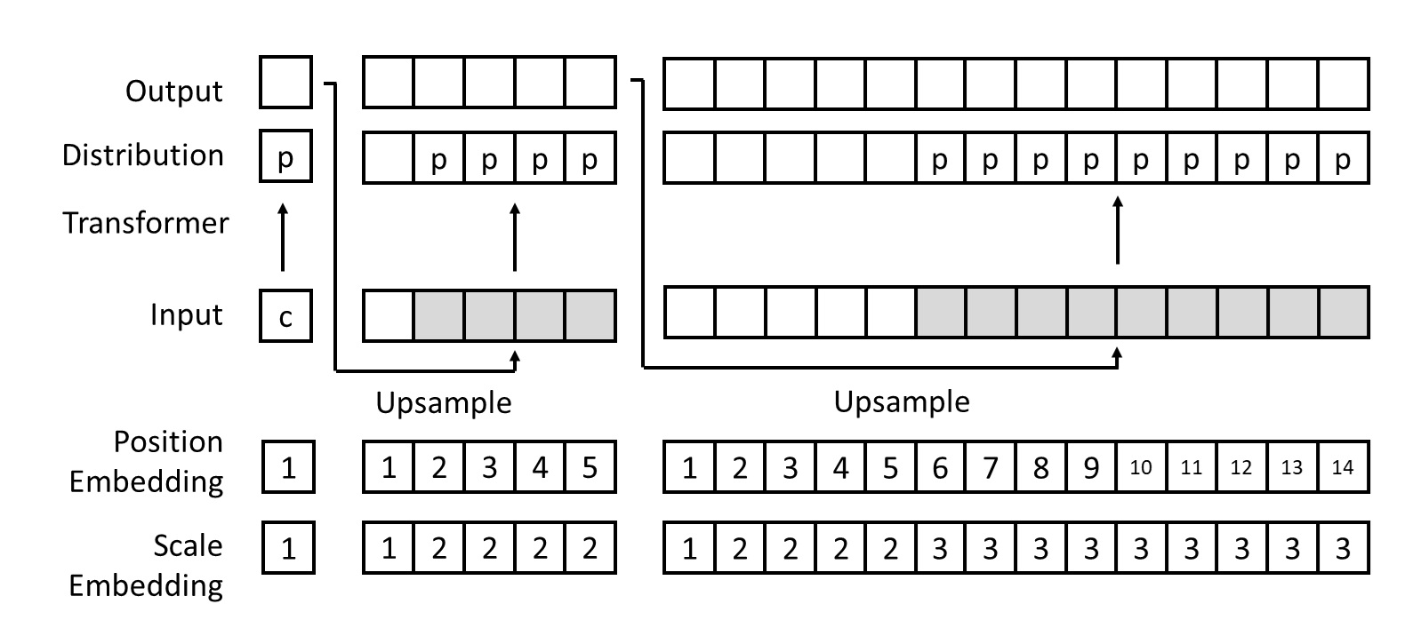
Once we have compressed the image into multi-scale token maps, the rest is straightforward. We simply flatten all tokens into a one-dimensional sequence and train a Transformer on that sequence. Since the task is now “next-scale prediction,” the model outputs the probability distributions for all tokens at the same scale in one loop, rather than merely the next token. Thus, even though the sequence becomes longer, the model is still faster overall because it can generate all tokens of a given scale in parallel. Meanwhile, the attention masking changes accordingly. Now, tokens at the same scale can see each other, but tokens at previous scales cannot see those at later scales. The following diagram illustrates the difference in attention masks and generation procedures for a
$3 \times 3$ token image under the “next-token” vs. “next-scale” approach.
In addition, the VAR Transformer also includes a few other modifications: 1) besides adding a 1D positional embedding to each token, tokens at the same scale share a scale embedding. All embeddings are learnable; 2) the Transformer and VQVAE decoder share the same embedding layer. Moreover, to reuse information from already generated images when creating a new scale, the initial embeddings for the new scale are obtained by performing bicubic upsampling on the previously generated results.
All other design elements of this Transformer are the same as those in VQGAN. For example, the Transformer has a decoder-only structure, and a special token is used at the first layer to encode the ImageNet class for class-conditional generation. The loss function is cross-entropy loss.
Quantitative Experiments on ImageNet
We have now seen most of the core aspects of VAR’s method. Let us briefly look at its experimental results. The paper claims that VAR performs well in both image generation and model scaling experiments. Specifically, VAR beats DiT in terms of FID score (Fréchet Inception Distance), and its generation speed is more than 45 times faster than DiT. Let us focus on VAR’s results on ImageNet $256 \times 256$ generation task. Below is a table from the paper. I have also included results from the MAR (Autoregressive Image Generation without Vector Quantization) by Kaiming He’s group .
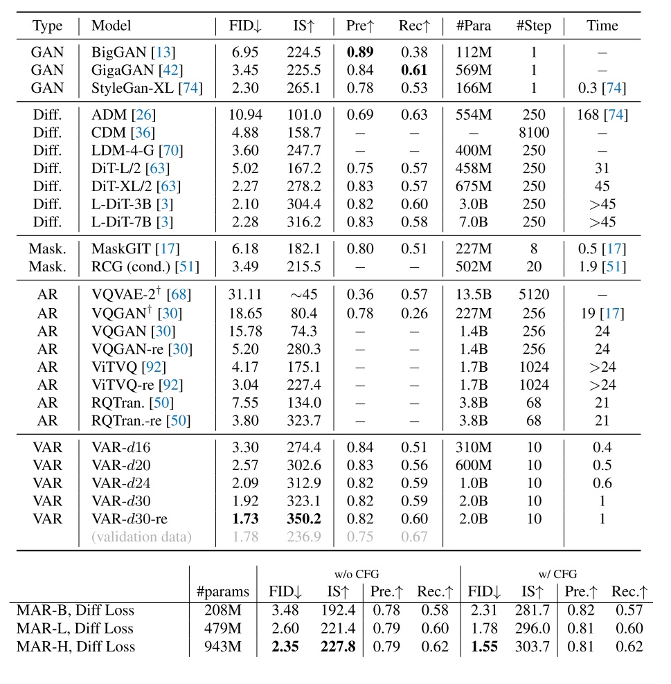
First, let’s compare DiT and VAR. In terms of speed, VAR is clearly much faster than DiT for any model size. In terms of FID as a measure of image quality, for the ~600M parameter regime, DiT still outperforms VAR. However, as the model size increases, DiT’s FID does not show improvement, whereas VAR’s FID keeps dropping. Eventually, VAR’s FID even surpasses that of the ImageNet validation set, at that point, there is little meaning in pushing FID any lower.
Then, let’s compare MAR and VAR. MAR can achieve an even more extreme FID (1.55) with a 943M model. But based on the MAR paper, its speed is about 5 times that of DiT-XL, meaning VAR is still faster—by a factor of around 9 compared to MAR.
On ImageNet, the FID of most SOTA models has essentially been maxed out. The main takeaway from the FID results is that VAR exhibits strong generative capabilities, on par with or better than DiT. However, for more challenging tasks like text-to-image, VAR’s performance is yet to be verified. Moreover, while DiT used 250 sampling steps to produce these benchmark numbers, in practical usage people usually sample in 20 steps. And with distillation, the sampling steps can be reduced to 4. Factoring in these acceleration techniques, VAR might not be faster than DiT.
Visualizing VAR’s Multi-Scale Generation
Having covered the main points of the paper, I will share some of my own theoretical analyses and experimental findings on VAR.
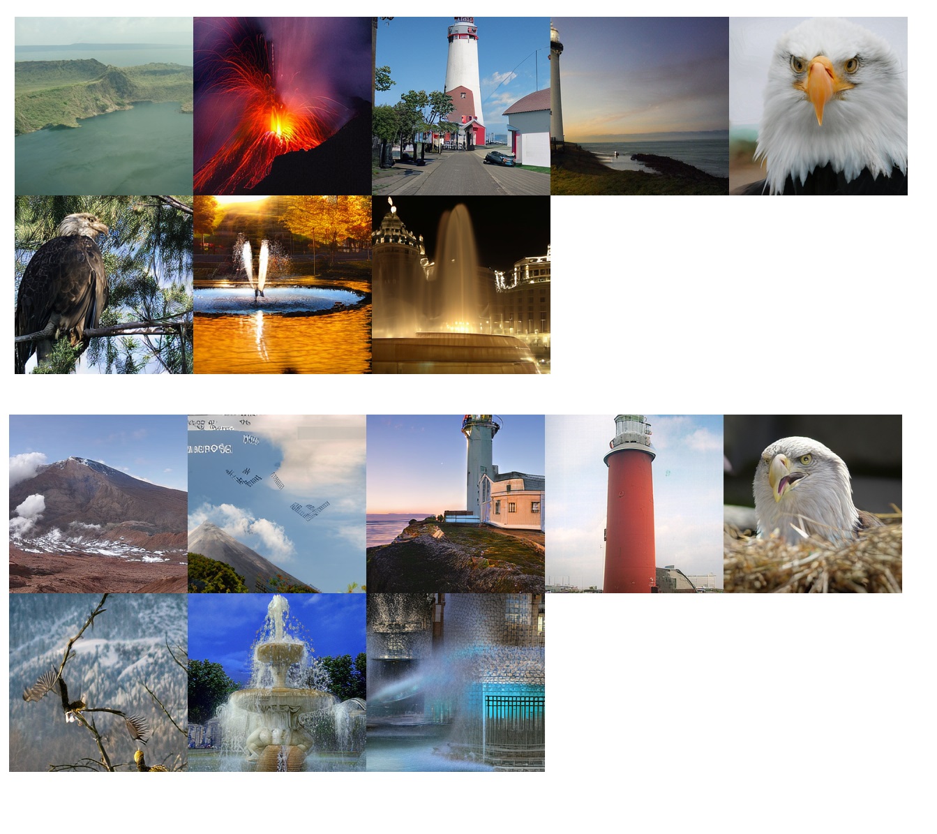
Let us look first at random sampling results. I used the largest VAR model with depth d=30. Under the default settings of the official sampling script, the outputs for two random seeds (0 and 15) are as shown below. The chosen ImageNet classes here are volcano, lighthouse, eagle, and fountain, with two images generated for each class. The generation is very fast, taking only about one second to produce all 8 images.
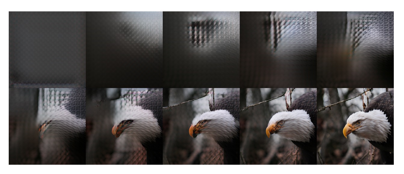
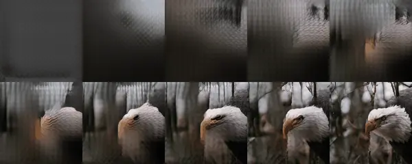
We can also observe the temporary images decoded at each scale after generation is completed. As expected, the image progresses from coarse to fine detail:
To further investigate which image components each scale is responsible for, we can do the following experiment: from a certain scale onward, switch to a different random seed generator. In GIF of each scale, the unchanged portions come from the earlier scales, and the varying parts come from the subsequent scales. As we can see, from around the third scale onward, the overall content of the image is essentially fixed—that is, structural information is determined in the first two scales. The further we go, the more image details are refined.
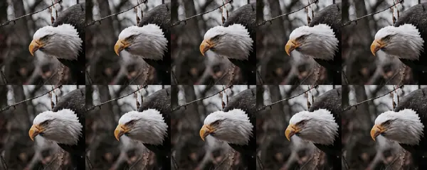
These results are rather surprising: does a $2 \times 2$ token map already determine the overall content of the image? Let us examine this in more detail.
Flaws in Single-Scale Generation
Some of you may feel something is off when studying VAR’s sampling algorithm: when generating the token map at a given scale, each token is sampled independently from a probability distribution.
According to the paper, VAR’s scale-autoregressive approach is a new autoregressive probabilistic model:
where $r_k$ denotes the token map at the $k$-th scale (from smallest to largest), and there are $K$ scales in total. Tokens in the same scale $r_k$ are generated in parallel. This means that during training (with a cross-entropy loss) and sampling, the method treats the probability of a token map as the product of the probabilities of all its tokens, assuming independence:
where $r_k^i$ is the $i$-th token at the $k$-th scale, and $I_k$ is the total number of tokens at that scale. I believe the above equation does not hold in principle. Even with the conditions imposed by previous scales, it is unlikely that the distributions for each token in the same scale are mutually independent. And as $I_k$ gets larger, the error introduced by that assumption grows.
Normally, independently sampling tokens at the same scale could result in inconsistencies in the generated image (like a “seam” every 16 pixels if each token represents a
$16 \times 16$ block). But why does VAR’s output still look coherent? On closer inspection of the VAR generation algorithm, we may find two features that greatly reduce discontinuities:
- VAR’s autoencoder uses vector quantization. This ensures the decoder’s input is always “reasonable,” and that the decoded image remains coherent.
- When generating a new scale, the model’s input is initialized with the bicubic upsampling of the previous scale’s image. This bicubic sampling ensures continuity among token embeddings.

Moreover, to further mitigate the negative effects of independent sampling, VAR effectively determines the image’s overall content by the time it completes the second or third scale; subsequent scales only refine image details. (Because as the number of tokens increases, the error from independent sampling grows). We have already verified this through the visualizations above. To show that only the first few scales matter, I did a bold experiment: after the Transformer generates the first two scales of tokens, I randomly generate all subsequent tokens. In the figure below, I froze the outputs of the first two scales and then generated multiple images with different random seeds for the later scales. The results show that if the first two scales are generated well, the rest of the tokens (even if sampled randomly) hardly affect the final image quality.
Based on these experiments, I think the real reason VAR works cannot be merely summarized as “next-scale prediction is a superior new generation paradigm.” The core success factor may be its multi-scale residual quantization autoencoder, which at least accomplishes the following:
- Uses vector quantization to ensure the decoder input is always valid.
- Adopts a multi-scale residual design, where each new scale’s token map not only records the information lost by downsampling but also the precision lost through vector quantization. Compared to a simple, human-interpretable Laplacian pyramid, this learnable degradation process may be more powerful.
- Performs bicubic upsampling of the lower-scale tokens, ensuring continuity in the generated images.
Of course, these components are entangled with one another. Without more in-depth experiments, we cannot pinpoint the single most crucial design element in VAR.
Multi-scale generation itself is not new—prior works like StyleGAN and Cascaded Diffusion have adopted similar strategies. However, VAR makes a bold choice: tokens within the same scale are sampled independently. Surprisingly, this mathematically questionable design does not severely degrade image quality. Thanks to this design, VAR can sample tokens within the same scale in parallel, drastically boosting generation speed.
Conclusions and Commentary
Previously, AR methods like VQGAN fell short in sampling speed and generation quality. The fundamental reasons are that next-token prediction for image tokens is both somewhat misguided and slow. To address this, VAR proposes a new AR strategy: decompose the latent into multiple scales, and generate the latent via next-scale prediction. To accommodate this, VAR modifies both the autoencoder and the Transformer used in VQGAN. In the autoencoder, images are encoded into multi-scale residual token maps, and in the Transformer, each scale’s tokens are assumed to have independent distributions. Experiments show that on ImageNet, VAR surpasses diffusion models like DiT in terms of image quality and is at least 45 times faster. Moreover, experiments suggest that VAR follows the scaling law.
From my perspective, as with other cutting-edge generative models, VAR has essentially maxed out ImageNet FID scores. Its performance on more challenging image-generation tasks remains to be proven. Recently, ByteDance released a text-to-image version of VAR called Infinity, but that model has not been open-sourced yet. We can continue to follow up on subsequent VAR-related work. As for speed, VAR may not be significantly faster than DiT once techniques such as reduced sampling steps and model distillation (for DiT) are applied. Of course, it is possible that VAR can be further accelerated in ways that have not been explored as extensively as with diffusion models.
Mathematically, the VAR approach has flaws: the token map’s distribution should not be the product of the independent distributions of its tokens. At least, the paper does not provide any analysis on this (nor does MAR, which uses a similar approach). Yet, simple generation experiments show that due to other designs that enforce continuity, the model outputs coherent images even if tokens at the same scale are sampled independently or even randomly. We need deeper experiments to really uncover why VAR is so effective.
I think if a research project could clearly explain which parts of VAR are making the biggest difference, retain those and discard the rest to propose a superior generation model, it would be a significant contribution. Potential directions for exploration include:
- Only the first few scales of tokens seem crucial in VAR. Perhaps we could generate those earlier scales using a more refined approach—for instance, a diffusion model—to ensure quality, while using a more efficient (maybe faster than a Transformer) model for the higher-scale token images. This could further enhance both quality and speed.
- VAR still relies on a VQ autoencoder, and no matter how you improve it, vector quantization reduces reconstruction accuracy. On the other hand, VQ can regularize the decoder’s input. Is it possible to replace VQ with VAE for its higher accuracy? And if so, how would we design a multi-scale encoding algorithm without VQ?